Getting started

The half-filled two-site Hubbard model is a compact many-body problem with hopping, local interactions, spin correlations, and an analytic solution. Its six-dimensional two-particle sector is small enough to inspect directly and already contains the charge-spin competition that appears throughout the repulsive Hubbard model.

The calculation below is fermionic. Bosonic calculations use the same sequence of sector construction, Hamiltonian diagonalization, and observable evaluation with bosonic basis states and commutation relations; worked examples are collected in Bosonic systems.

The Hamiltonian is

\[ H=-t\sum_{\sigma} \left(c_{0\sigma}^\dagger c_{1\sigma}+c_{1\sigma}^\dagger c_{0\sigma}\right) +U\sum_{i=0}^{1} n_{i\uparrow}n_{i\downarrow}, \]

Here \(c_{i\sigma}^\dagger\) and \(c_{i\sigma}\) create and annihilate a fermion with spin \(\sigma\) on site \(i\). The number operator is \(n_{i\sigma}=c_{i\sigma}^\dagger c_{i\sigma}\), \(t\) is the nearest-neighbor hopping amplitude, and \(U\) is the on-site repulsion. The calculation uses \(t=1\) as the energy unit, \(U/t=4\), and two fermions.

Installation

Install EDinPy from a source checkout:

git clone https://github.com/QuantumArtificer/edinpy.git
cd edinpy
python -m pip install -e .

Verify the import:

import edinpy
print(edinpy.__version__)

0.3.0

1. Define the fermionic modes

A spinful site contributes two fermionic modes, one for each spin component. The site and spin labels define the ordered one-particle basis:

from edinpy import fermion as edf

site = edf.DoF(2, name="site")
spin = edf.DoF(2, name="spin")
modes = edf.FermionModes(site, spin)

print("number of modes:", modes.n_modes)
for p in range(modes.n_modes):
    print(p, modes.unravel(p))

number of modes: 4
0 (0, 0)
1 (1, 0)
2 (0, 1)
3 (1, 1)

The first degree of freedom is the fastest-varying index. With FermionModes(site, spin), the canonical ordering is therefore

\[ (0,\uparrow),\ (1,\uparrow),\ (0,\downarrow),\ (1,\downarrow). \]

This ordering fixes the occupation-bit convention and therefore the signs of fermionic creation and annihilation operators. The ordering is part of the definition of the calculation.

2. Choose the fixed-particle-number sector

At half filling the dimer contains two fermions:

sector = edf.NParticleSector(modes, N=2).build()
print("dimension:", sector.dimension)
print("basis bit strings:", sector.basis.states)

dimension: 6
basis bit strings: (3, 5, 6, 9, 10, 12)

The dimension is

\[ \dim \mathcal H_{N=2}=\binom{4}{2}=6. \]

FockBasis stores each occupation configuration as an integer bit string. The basis is ordered by that integer representation.

3. Choose the notation

Bind the primitive operator classes to the mode set and choose the notation used in the script:

c = edf.set_notation(edf.Annihilation, modes)
cd = edf.set_notation(edf.Creation, modes)
n = edf.set_notation(edf.Number, modes)

UP, DOWN = 0, 1

print(c(1, DOWN))
print(cd(0, UP))
print(n(0, UP))

c[1,1]
c†[0,0]
n[0,0]

The bound names retain the labels and ordering defined by modes, so operator expressions stay close to the second-quantized notation used for the model.

4. Write the Hamiltonian literally

t = 1.0
U = 4.0
H = 0

for sigma in (UP, DOWN):
    H += -t * (
        cd(0, sigma) * c(1, sigma)
        + cd(1, sigma) * c(0, sigma)
    )

for i in range(2):
    H += U * n(i, UP) * n(i, DOWN)

print(H)

-1.0 c†[0,0] c[1,0] + -1.0 c†[1,0] c[0,0] + -1.0 c†[0,1] c[1,1] + -1.0 c†[1,1] c[0,1] + 4.0 n[0,0] n[0,1] + 4.0 n[1,0] n[1,1]

At this stage H is still a second-quantized operator expression. Its numerical representation is introduced when the expression is combined with the finite sector.

The literal expression exposes the model term by term. The standard helpers Hopping and Hubbard construct the same physical terms when a compact form is useful.

5. Inspect the many-body matrix

import numpy as np

hamiltonian = edf.Hamiltonian(H, sector)
np.set_printoptions(precision=3, suppress=True)

print("shape:", hamiltonian.matrix.shape)
print("dtype:", hamiltonian.matrix.dtype)
print("nnz:", hamiltonian.matrix.nnz)
print(hamiltonian.toarray())

shape: (6, 6)
dtype: float64
nnz: 10
[[ 0.  0.  0.  0.  0.  0.]
 [ 0.  4. -1. -1.  0.  0.]
 [ 0. -1.  0.  0. -1.  0.]
 [ 0. -1.  0.  0. -1.  0.]
 [ 0.  0. -1. -1.  4.  0.]
 [ 0.  0.  0.  0.  0.  0.]]

The matrix is sparse even in this tiny example. The interaction is diagonal. Hopping connects only occupation states related by moving one fermion.

6. Solve the eigensystem

For a six-dimensional example it is useful to request the complete spectrum:

energies, eigenvectors = hamiltonian.eigsolve(k=None)
print(energies)

[-0.82842712  0.          0.          0.          4.          4.82842712]

The threefold level at zero is the spin-triplet manifold. The interacting singlet is the ground state.

For larger sparse problems, request only the part of the spectrum needed for the calculation:

energies, eigenvectors = hamiltonian.eigsolve(k=4, which="SA")

which="SA" follows the SciPy/ARPACK convention and requests the smallest algebraic eigenvalues.

7. Recover the ground-state ket

The columns returned by eigsolve are NumPy arrays in sector.basis ordering. Hamiltonian.eigenstate() returns the same eigenvector as a basis-aware FockVector:

psi0 = hamiltonian.eigenstate(0)

print("norm:", psi0.norm())
print("bra-ket:", psi0.dag * psi0)

norm: 0.9999999999999999
bra-ket: 0.9999999999999998

Floating-point roundoff at the \(10^{-16}\) level is expected. The returned eigenstate participates directly in the same literal algebra as the operators, which makes bra-ket expectation values and custom observables natural to write.

Before calculating observables, it is useful to look at the state itself. The coefficient vector follows sector.basis order:

for state, coefficient in zip(sector.basis.states, psi0.coefficients):
    print(f"|{state:04b}>  {coefficient.real: .8f}")

|0011>   0.00000000
|0101>  -0.27059805
|0110>  -0.65328148
|1001>  -0.65328148
|1010>  -0.27059805
|1100>   0.00000000

The bit strings use the canonical mode ordering defined above. The dominant configurations are the two singly occupied states with opposite spins. The doublon-holon configurations remain present with smaller weight because \(U/t=4\) is strongly correlated but not the \(U/t\to\infty\) limit.

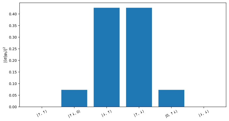
Ground-state probability in each physical occupation configuration at \(U/t=4\). The antiferromagnetically correlated singly occupied configurations dominate, while finite hopping retains a smaller doublon-holon component.

8. Calculate observables with Dirac algebra

The total double-occupancy operator is

\[ D=n_{0\uparrow}n_{0\downarrow}+n_{1\uparrow}n_{1\downarrow}. \]

Construct and print it:

D = sum(
    (n(i, UP) * n(i, DOWN) for i in range(2)),
    start=0,
)

print(D)

n[0,0] n[0,1] + n[1,0] n[1,1]

Then write the expectation value exactly as in Dirac notation:

double_occupancy = psi0.dag * D * psi0
print(double_occupancy)

0.1464466094067262

The method form is also available when it is convenient in algorithmic code:

print(psi0.inner(D * psi0))

0.1464466094067262

psi0.dag * D * psi0 is the preferred form when writing physics. The same state-operator product works for any operator expression that acts within the represented sector.

9. Connect the observables to the exact dimer physics

Introduce

\[ R=\sqrt{U^2+16t^2}. \]

For the symmetric half-filled dimer the exact ground-state energy is

\[ E_0=\frac{U-R}{2}. \]

The Hellmann-Feynman theorem gives the total double occupancy

\[ \langle D\rangle =\frac{\partial E_0}{\partial U} =\frac{1}{2}\left(1-\frac{U}{R}\right). \]

A complementary local-spin diagnostic is the site-averaged local moment

\[ \mu^2=\frac{1}{2}\sum_{i=0}^{1} \left\langle(n_{i\uparrow}-n_{i\downarrow})^2\right\rangle. \]

At half filling, \(\mu^2=1-\langle D\rangle\). The spin correlation follows

\[ \langle\mathbf S_0\cdot\mathbf S_1\rangle =-\frac{3}{4}\mu^2, \]

and the lowest singlet-triplet excitation gap is

\[ \Delta_{ST}=\frac{R-U}{2} \xrightarrow[U/t\gg1]{}\frac{4t^2}{U}. \]

The corresponding EDinPy operators are still ordinary symbolic expressions:

local_moment = 0.5 * sum(
    (n(i, UP) - n(i, DOWN)) * (n(i, UP) - n(i, DOWN))
    for i in range(2)
)
S01 = edf.HeisenbergExchange(
    (0, UP), (0, DOWN),
    (1, UP), (1, DOWN),
    J=1.0,
    modes=modes,
)

print("<D> =", psi0.dag * D * psi0)
print("mu^2 =", psi0.dag * local_moment * psi0)
print("<S0.S1> =", psi0.dag * S01 * psi0)
print("Delta_ST =", energies[1] - energies[0])

<D> = 0.1464466094067262
mu^2 = 0.8535533905932736
<S0.S1> = -0.6401650429449552
Delta_ST = 0.8284271247461903

Repulsion first suppresses the charge fluctuations carried by doublon-holon configurations.

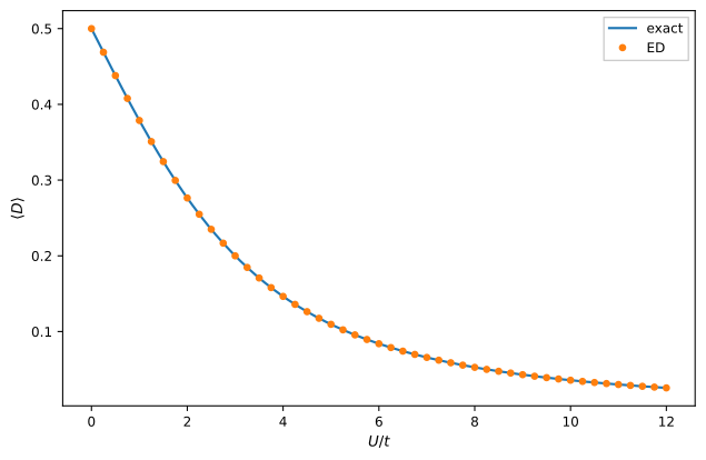
Total double occupancy of the half-filled dimer. Exact diagonalization follows the analytic result as the doublon-holon component is suppressed with increasing \(U/t\).

The same redistribution increases the weight of the singly occupied singlet sector and drives the bond correlation toward the two-spin value \(-3/4\).

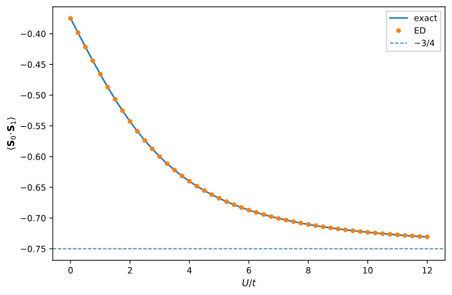
Ground-state bond spin correlation. The strong-coupling limit approaches the spin singlet value \(\langle\mathbf S_0\!\cdot\!\mathbf S_1\rangle=-3/4\).

Charge fluctuations remain virtually active at large \(U/t\), producing the antiferromagnetic superexchange scale.

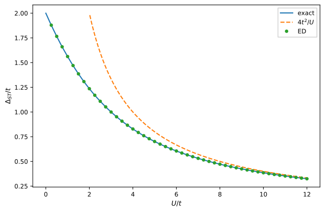
Singlet-triplet gap of the Hubbard dimer. The exact result approaches \(4t^2/U\) once the charge excitation scale is large compared with the hopping.

The Hubbard dimer is a standard analytic many-body benchmark. Carrascal et al. give a detailed treatment of its exact solution and correlation physics in J. Phys.: Condens. Matter 27, 393001 (2015), doi:10.1088/0953-8984/27/39/393001.

The full Hubbard dimer: charge fluctuations and superexchange example develops these relations in more detail.

10. Perform a numerical sanity check

A residual checks the eigensolver independently of physical interpretation:

residual = np.linalg.norm(
    hamiltonian.matrix @ eigenvectors[:, 0]
    - energies[0] * eigenvectors[:, 0]
)
print(residual < 1e-10)

True

The residual measures the numerical consistency of the returned eigenpair. Physical validation comes from the model definition, boundary conditions, analytic limits, symmetry checks, and finite-size analysis appropriate to the problem.

Where to go next

Further details on sectors, operator algebra, eigensolvers, and observables are collected in the User guide. The Hubbard dimer: charge fluctuations and superexchange, Half-filled Hubbard ring: Mott correlations on a finite cluster, and Bosonic systems calculations continue with larger fermionic and bosonic systems. Function and class signatures are collected in API reference.