Half-filled Hubbard ring: Mott correlations on a finite cluster

The one-dimensional repulsive Hubbard model is a standard setting for the interplay between itinerancy, local-moment formation, and antiferromagnetic correlations. At half filling the thermodynamic chain is insulating for every \(U>0\) by the Lieb-Wu solution.[1] A finite ring does not exhibit a thermodynamic transition, but it resolves how charge fluctuations are suppressed and how spin correlations become increasingly dominant as \(U/t\) grows.

For a periodic ring of \(L=6\) sites,

\[ H=-t\sum_{i,\sigma} \left(c_{i\sigma}^\dagger c_{i+1,\sigma}+\mathrm{H.c.}\right) +U\sum_i n_{i\uparrow}n_{i\downarrow}, \]

with \(c_{L\sigma}=c_{0\sigma}\) and \(N=L=6\). The fixed-\(N\) Hilbert space contains

\[ \binom{12}{6}=924 \]

states.

Ground state and low-energy spectrum

import numpy as np
from edinpy import fermion as edf

L = 6
UP, DOWN = 0, 1

site = edf.DoF(L, name="site")
spin = edf.DoF(2, name="spin")
modes = edf.FermionModes(site, spin)
sector = edf.NParticleSector(modes, N=L).build()

c = edf.set_notation(edf.Annihilation, modes)
cd = edf.set_notation(edf.Creation, modes)
n = edf.set_notation(edf.Number, modes)

H = 0
for i in range(L):
    j = (i + 1) % L
    for sigma in (UP, DOWN):
        hop = cd(i, sigma) * c(j, sigma)
        H += -(hop + hop.dag)
    H += 4.0 * n(i, UP) * n(i, DOWN)

hamiltonian = edf.Hamiltonian(H, sector)
energies, _ = hamiltonian.eigsolve(k=8, which="SA")
psi0 = hamiltonian.eigenstate(0)

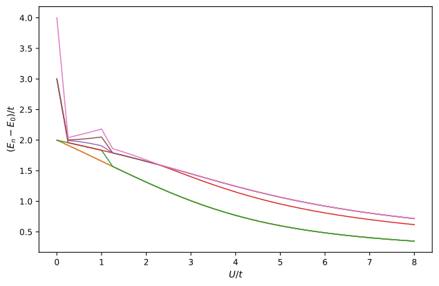
Lowest excitation energies of the half-filled six-site ring. Interaction reorganizes the low-energy manifold continuously on the finite cluster; the decreasing spin scale at large \(U/t\) is consistent with the emergence of an exchange scale proportional to \(t^2/U\).

Local charge fluctuations and moment formation

The site-averaged double occupancy is

\[ D=\frac1L\sum_i \langle n_{i\uparrow}n_{i\downarrow}\rangle, \]

while the local moment is

\[ \mu^2=\frac1L\sum_i \left\langle(n_{i\uparrow}-n_{i\downarrow})^2\right\rangle. \]

def double_occupancy(psi):
    return sum(
        np.real(psi.dag * n(i, UP) * n(i, DOWN) * psi)
        for i in range(L)
    ) / L


def local_moment(psi):
    return sum(
        np.real(
            psi.dag
            * (n(i, UP) - n(i, DOWN))
            * (n(i, UP) - n(i, DOWN))
            * psi
        )
        for i in range(L)
    ) / L

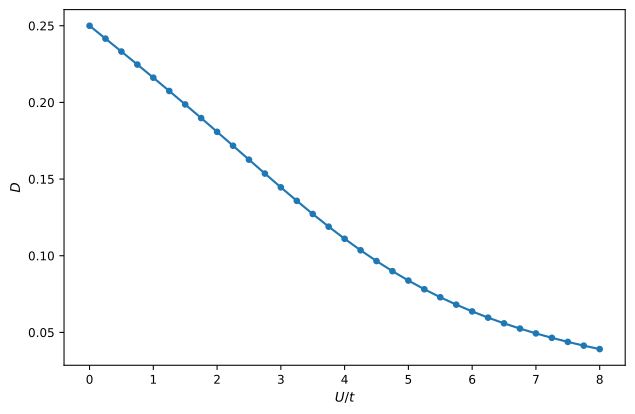
Site-averaged double occupancy. Increasing repulsion suppresses local charge fluctuations and transfers weight toward singly occupied configurations.

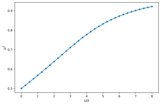
Site-averaged local moment. The growth of \(\mu^2\) accompanies the loss of doublon weight and marks the formation of well-defined local spins on the finite ring.

Real-space correlations

Define

\[ S_i^z=\frac12(n_{i\uparrow}-n_{i\downarrow}), \qquad \delta n_i=n_i-1, \]

and translationally averaged equal-time correlations

\[ C_s(r)=\frac1L\sum_i\langle S_i^zS_{i+r}^z\rangle, \qquad C_c(r)=\frac1L\sum_i\langle\delta n_i\delta n_{i+r}\rangle. \]

With the local spin and charge operators defined explicitly, the correlation function is

spin_z = [edf.SpinZ((i, UP), (i, DOWN), modes) for i in range(L)]
delta_n = [n(i, UP) + n(i, DOWN) - 1 for i in range(L)]


def correlation(psi, operators, r):
    return sum(
        np.real(psi.dag * operators[i] * operators[(i + r) % L] * psi)
        for i in range(L)
    ) / L

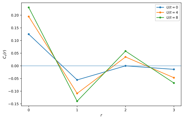
Spin correlations on the half-filled ring. Repulsion strengthens the alternating sign pattern expected from antiferromagnetic correlations at half filling.

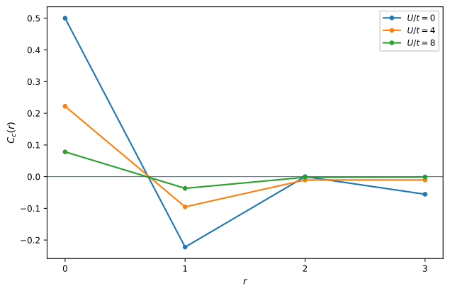
Connected charge correlations on the same ring. Their amplitude decreases as double occupancy is suppressed and charge motion becomes increasingly costly.

Momentum-space structure factors

For local operators \(O_j\), define

\[ O_q=\sum_j e^{-iqj}O_j, \qquad S_O(q)=\frac1L\langle O_q^\dagger O_q\rangle. \]

In code,

def structure_factor(psi, operators, q):
    Oq = sum(
        (np.exp(-1j * q * j) * op for j, op in enumerate(operators)),
        start=0,
    )
    return np.real(psi.dag * Oq.dag * Oq * psi) / L

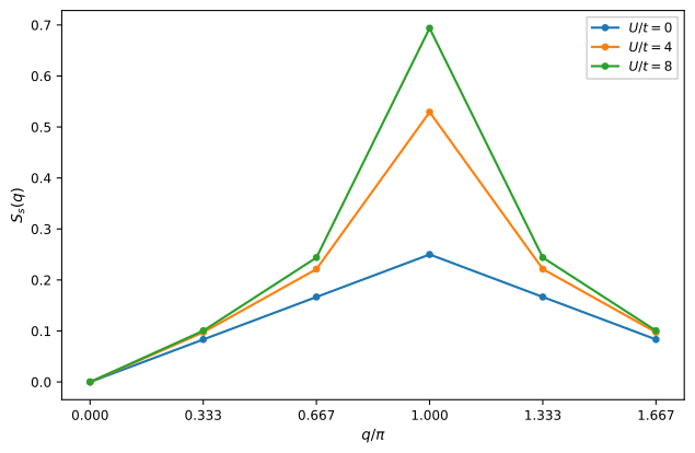
Spin structure factor. The \(q=\pi\) response grows with repulsion, reflecting the increasingly staggered spin correlations of the half-filled ring.

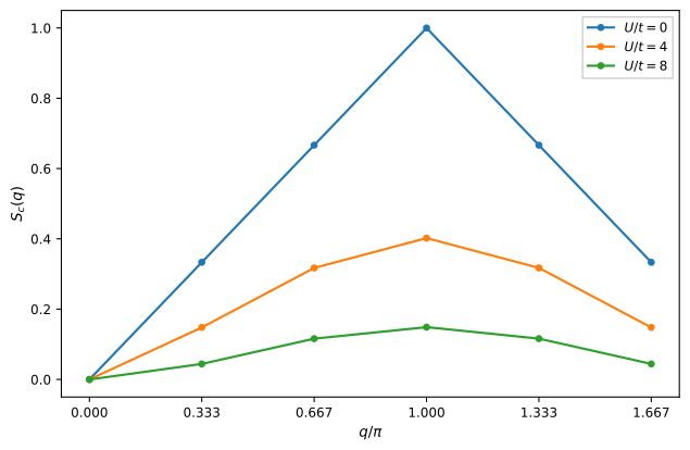
Charge structure factor. Repulsion suppresses the staggered charge response relative to the noninteracting ring.

For onsite singlet pairs,

\[ \Delta_i=c_{i\downarrow}c_{i\uparrow}, \]

and

\[ P(q)=\frac1L\langle\Delta_q^\dagger\Delta_q\rangle. \]

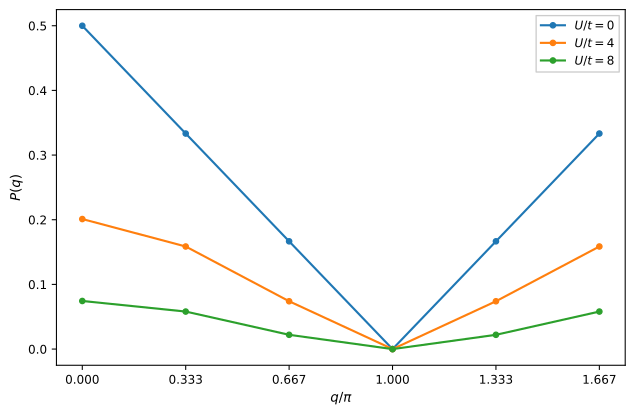
Onsite pair structure factor. Repulsive \(U\) suppresses onsite pairing correlations throughout momentum space.

The real-space and momentum-space observables give a consistent finite-cluster picture. Increasing \(U/t\) suppresses doublons and connected charge fluctuations while strengthening the staggered spin response. The onsite pair channel is suppressed at the same time. These trends diagnose the redistribution of low-energy weight on the finite ring; they do not by themselves establish a thermodynamic order parameter.

Finite-size sequence

Finite-size dependence can be examined without changing the model. For even open chains at half filling, the ground state lies in the \(S_z=0\) sector, so fixing

\[ N_\uparrow=N_\downarrow=L/2 \]

reduces the basis before diagonalization. A compact size sweep is

def open_chain_energy_density(L, U=4.0, t=1.0):
    site = edf.DoF(L, name="site")
    spin = edf.DoF(2, name="spin", labels=("up", "down"))
    modes = edf.FermionModes(site, spin)
    sector = (
        edf.NParticleSector(modes, N=L)
        .project_particles("spin", up=L // 2, down=L // 2)
        .build()
    )

    c = edf.set_notation(edf.Annihilation, modes)
    cd = edf.set_notation(edf.Creation, modes)
    n = edf.set_notation(edf.Number, modes)

    H = 0
    for i in range(L - 1):
        for sigma in (UP, DOWN):
            hop = cd(i, sigma) * c(i + 1, sigma)
            H += -t * (hop + hop.dag)
    for i in range(L):
        H += U * n(i, UP) * n(i, DOWN)

    ham = edf.Hamiltonian(H, sector)
    E, _ = ham.eigsolve(k=1, which="SA", tol=1e-10)
    return E[0] / (L * t)


sizes = (4, 6, 8, 10)
energy_density = [open_chain_energy_density(L) for L in sizes]

At \(U/t=4\), the Lieb-Wu thermodynamic result can be written

\[ \frac{E_0}{Lt}\bigg|_{L\to\infty} =-4\int_0^\infty \frac{J_0(\omega)J_1(\omega)} {\omega\left(1+e^{2\omega}\right)}\,d\omega \simeq -0.573729. \]

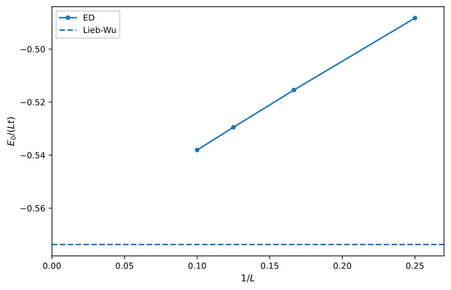
Ground-state energy density at \(U/t=4\) for even open chains. The finite-system values move toward the Lieb-Wu thermodynamic result as \(1/L\) decreases.

The energy density is already smooth over this short sequence, but that behavior cannot be transferred automatically to gaps or correlation functions. Different observables can carry different finite-size corrections, and periodic clusters can show additional shell effects.

---

[1]

E. H. Lieb and F. Y. Wu, “Absence of Mott Transition in an Exact Solution of the Short-Range, One-Band Model in One Dimension,” Phys. Rev. Lett. 20, 1445 (1968), doi:10.1103/PhysRevLett.20.1445.