Schwinger bosons for a spin-1/2 Heisenberg dimer#

The Schwinger-boson representation replaces a local spin by two bosonic modes.[1][2]

\[ S_i^+=b_{i\uparrow}^\dagger b_{i\downarrow},\qquad S_i^-=b_{i\downarrow}^\dagger b_{i\uparrow},\qquad S_i^z=\frac12(n_{i\uparrow}-n_{i\downarrow}). \]

The local constraint

\[ n_{i\uparrow}+n_{i\downarrow}=2S \]

selects the physical spin-\(S\) representation. For \(S=1/2\), one boson per site gives two local states and reproduces the ordinary spin-\(1/2\) algebra.

For two sites,

\[ H=J\,\mathbf S_0\cdot\mathbf S_1. \]

Constrained bosonic Hilbert space#

from edinpy import boson as edb

site = edb.DoF(2, name="site", labels=("left", "right"))
component = edb.DoF(2, name="component", labels=("up", "down"))
modes = edb.BosonModes(site, component)

sector = (
    edb.NParticleSector(modes, N=2)
    .project_particles("site", left=1, right=1)
    .build()
)

The constraint leaves four states, exactly the Hilbert space of two spin-\(1/2\) degrees of freedom.

UP, DOWN = 0, 1
Sdot = edb.HeisenbergExchange(
    (0, UP), (0, DOWN),
    (1, UP), (1, DOWN),
    J=1.0,
    modes=modes,
)

The analytic spectrum is

\[ E_{S=0}=-\frac{3J}{4},\qquad E_{S=1}=\frac{J}{4}. \]

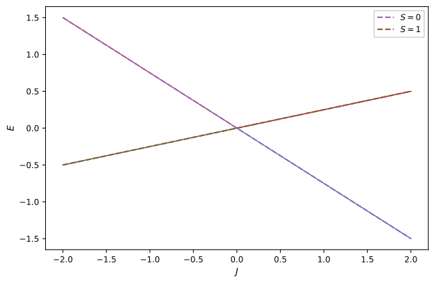
Singlet and triplet energies of a Schwinger-boson Heisenberg dimer — Schwinger-boson spectrum of the locally constrained Heisenberg dimer. The bosonic representation reproduces the singlet and triplet branches exactly.#

Total-spin operator#

The total-spin Casimir is

\[ \mathbf S_{\mathrm{tot}}^2 =(S_{\mathrm{tot}}^z)^2 +\frac12\left(S_{\mathrm{tot}}^+S_{\mathrm{tot}}^-+S_{\mathrm{tot}}^-S_{\mathrm{tot}}^+\right). \]

Splus = sum(
    (edb.SpinPlus((i, UP), (i, DOWN), modes) for i in range(2)),
    start=0,
)
Sminus = sum(
    (edb.SpinMinus((i, UP), (i, DOWN), modes) for i in range(2)),
    start=0,
)
Sz = sum(
    (edb.SpinZ((i, UP), (i, DOWN), modes) for i in range(2)),
    start=0,
)
S2 = Sz * Sz + 0.5 * (Splus * Sminus + Sminus * Splus)

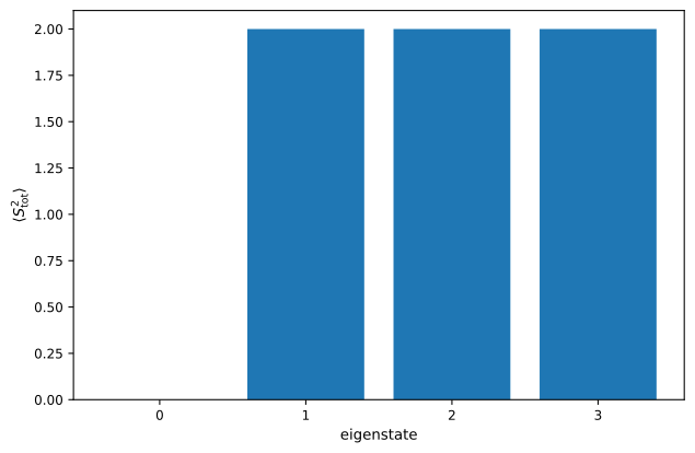
Total spin squared for the four eigenstates of the Schwinger-boson Heisenberg dimer — Total-spin diagnostic at \(J=1\). The ground-state singlet has \(S(S+1)=0\) and the triplet manifold has \(S(S+1)=2\).#

The local occupancy constraint removes the unphysical bosonic states and leaves precisely the spin-\(1/2\) Hilbert space.