Benchmark matrix

The publication suite is deliberately broader than a collection of smooth Gaussian tests. It combines localized fields with different regularity and angular content, 13 physical kernel parameterizations spanning ten families, plus one smooth numerical control, and displacement ranges that span four decades.

The same definitions are used throughout the documentation when a method is described as suitable for a particular class of inputs.

Numerical targets used by the publication suite

Every tolerance quoted in the documentation is attached to a specific numerical control. The publication suite uses the following targets.

Study	Requested quantity	Values
HarmonicTransform tolerance response	HarmonicTransform.rtol	1e-3, 1e-4, 1e-5
HarmonicTransform automatic convergence	HarmonicTransform.rtol	1e-4
HarmonicTransform q-support search	HarmonicTransform.q_tail_rtol	1e-3
Interaction broad accuracy response	Interaction.rtol	1e-3, 1e-4, 1e-5
Interaction public-method matrix	Interaction.rtol	1e-4
Interaction canonical automatic convergence	Interaction.rtol	1e-4
Interaction practical large-displacement study	Interaction.rtol	1e-3
Large-displacement independent-reference stability	reference_required_max_change	1e-5

The automatic selectors use HarmonicTransform.atol = 1e-12 and Interaction.atol = 1e-12 as absolute floors. Numerical tolerances are reported together with their parameter names because rtol, q_tail_rtol, and atol control distinct numerical tests. In particular, rtol is a self-convergence threshold on successive numerical results; it is not a pointwise relative-error bound. Independent validation is reported with global relative \(L^2\) and peak-normalized maximum errors as defined in Accuracy and automatic convergence.

Smooth Gaussian family

The smooth reference family is built from

(1)\[g_0(r)=e^{-r^2},\qquad g_1(r)=r e^{-r^2},\qquad g_2(r)=r^2 e^{-r^2},\qquad g_4(r)=r^4 e^{-r^2}.\]

Their analytic Hankel transforms are

(2)\[G_0(q)=\frac12e^{-q^2/4},\quad G_1(q)=\frac{q}{4}e^{-q^2/4},\quad G_2(q)=\frac{q^2}{8}e^{-q^2/4},\quad G_4(q)=\frac{q^4}{32}e^{-q^2/4}.\]

The suite uses an isotropic \(m=0\) field, an odd conjugate pair \(m=\pm1\), an anisotropic \(m=0,\pm2\) field, and a five-harmonic \(m=0,\pm2,\pm4\) field. These cases represent the smooth, rapidly localized inputs for which the default finite quadratures are intended.

Nodal and complex fields

The nodal benchmark adds

(3)\[n_0(r)=(1-r^2)e^{-r^2},\qquad N_0(q)=\frac{q^2}{8}e^{-q^2/4},\]

with smaller \(m=\pm2\) Gaussian components. The complex mixed-parity field is

(4)\[\rho(r,\theta)= g_0(r) +0.35e^{0.4i}g_1(r)e^{i\theta} +0.20e^{-0.7i}g_2(r)e^{-2i\theta}.\]

The latter contains odd and even differences \(m-m'\) and is therefore sensitive to the signed-order Bessel parity in the translated four-center integral.

Difficult radial profiles

Three workloads are marked as difficult in the interaction benchmark definition:

(5)\[c(r)=e^{-r},\qquad o(r)=e^{-0.35r}\cos(5r),\qquad a_0(r)=(1+r^2)^{-2}.\]

The algebraic workload also contains

(6)\[a_2(r)=\frac{r^2}{(1+r^2)^{7/2}}.\]

Their analytic transforms are used to qualify HarmonicTransform independently of the later interaction integral. These profiles probe a cusp, radial oscillations, and a long algebraic tail. They should not be interpreted as failures of a method when a parameter box that works well for smooth localized inputs is deliberately refused.

The harmonic benchmark also contains discontinuous top-hat and annular stress tests. Automatic refusal is the expected outcome for those stress profiles at the declared settings.

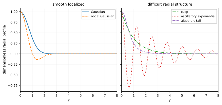
Representative radial functions from the publication suite. The Gaussian and nodal profiles decay rapidly and are smooth. The cusp has a non-smooth derivative at the origin, the oscillatory exponential contains several radial sign changes before decaying, and the algebraic profile retains a substantially longer tail. These distinctions are used throughout the User Guide when separating ordinary localized inputs from difficult radial structure.

Kernel families

The interaction suite uses the momentum-space convention described in Fourier and coordinate conventions. Overall electrostatic prefactors are fixed to \(2\pi\) because the benchmark measures relative numerical errors.

The tested kernels include the Rytova–Keldysh thin-film family [Keldysh, 1979, Rytova, 1967] together with the other radial forms below:

(7)\[\begin{split}\begin{aligned} U_{\mathrm C}(q) &= \frac{2\pi}{q},\\ U_{\mathrm{RK}}(q) &= \frac{2\pi}{q(1+r_0q)},\\ U_{\mathrm{dual}}(q) &= \frac{2\pi\tanh(qd)}{q},\\ U_{\mathrm{single}}(q) &= \frac{2\pi[1-e^{-2qd}]}{q},\\ U_{\mathrm{TF}}(q) &= \frac{2\pi}{q+q_{\mathrm{TF}}},\\ U_{\mathrm Y}(q) &= \frac{2\pi}{\sqrt{q^2+\kappa^2}},\\ U_{\mathrm H}(q) &= \frac{2\pi}{q^2+\kappa^2},\\ U_{\mathrm{inter}}(q) &= \frac{2\pi e^{-qd}}{q},\\ U_{\mathrm{gated\ inter}}(q) &= \frac{2\pi e^{-qd_{\ell}}\tanh(qd_g)}{q}. \end{aligned}\end{split}\]

The benchmark values are \(r_0=0.1,1,10\), \(d=1\), \(q_{\mathrm{TF}}=1\), \(\kappa=0.1,1,10\), and \(d_{\ell}=d_g=1\) where applicable.

The static zero-temperature 2DEG RPA kernel uses Stern’s polarizability [Stern, 1967] and is

(8)\[U_{\mathrm{RPA}}(q)=\frac{2\pi}{q+q_{\mathrm{TF}}F(q)},\]

with \(k_F=q_{\mathrm{TF}}=1\) and

(9)\[\begin{split}F(q)= \begin{cases} 1, & q\le2k_F,\\ 1-\sqrt{1-(2k_F/q)^2}, & q>2k_F. \end{cases}\end{split}\]

The nonanalytic point at \(q=2k_F\) is supplied explicitly to the independent reference quadrature. A smooth Gaussian kernel \(U(q)=2\pi e^{-q^2/8}\) is included only as a numerical control.

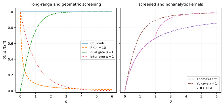
Representative benchmark kernels plotted as \(qU(q)/(2\pi)\) so the Coulomb singularity at \(q=0\) does not dominate the scale. Coulomb is constant in this representation. Rytova-Keldysh and interlayer screening suppress large q, gate-screened and Thomas-Fermi forms remove the Coulomb divergence at small q, and the 2DEG RPA curve carries the \(2k_F\) nonanalyticity used to test piecewise reference integration.

The 74-case Interaction matrix

The broad Interaction benchmark at Interaction.rtol = 1e-4 contains 74 distinct field/kernel combinations:

Group	Construction	Cases
continuity	all nine non-stress field workloads with \(r_0=1\) Rytova-Keldysh screening	9
kernel sweep	four representative fields crossed with 13 physical kernels	52
difficult fields	cusp, oscillatory exponential, and algebraic fields with four representative kernels	12
smooth control	complex mixed-parity field with the Gaussian numerical-control kernel	1
total		74

The four representative fields are the isotropic Gaussian, anisotropic \(m=0,\pm2\) Gaussian, nodal mixed field, and complex mixed-parity field. The difficult-field group is intentionally smaller because its role is to stress radial behavior, not to multiply every kernel by every profile.

Displacement regimes

The displacement magnitude \(\delta=|\boldsymbol\Delta|\) is measured in the same length unit as the input orbital coordinates. The standard interaction domain is

(10)\[10^{-2}\le\delta\le10^2,\]

and the large-displacement domain is

(11)\[10^2\le\delta\le10^4.\]

Thus the upper endpoint \(\delta=10^4\) means a separation of \(10^4\) in that same represented length unit. The large-displacement regime is numerically different because the translation Bessel functions oscillate rapidly across the represented q interval. Recommendations for this regime are separated explicitly in Choosing numerical methods and Convergence and diagnostics.

Canonical automatic-convergence cases

The stricter automatic-convergence study uses four cases that deliberately combine different field and kernel features:

Case	Field	Kernel	Feature being exercised
isotropic_coulomb	isotropic Gaussian	Coulomb	singular kernel, one harmonic
anisotropic_rk_strong	\(m=0,\pm2\) Gaussian	RK with \(r_0=10\)	anisotropy and strong screening
complex_gate	complex mixed parity	dual gate	complex odd/even angular coupling
nodal_rpa	nodal mixed	2DEG RPA	nodal field plus \(2k_F\) nonanalyticity

Every automatically accepted result from these cases is checked against an independent reference after parameter selection. Selector acceptance and independent reference accuracy are reported separately in Accuracy and automatic convergence.