Performance and scaling

Performance measurements are reported only for numerical states whose accuracy status is known. Calibration and fixed production are timed separately. The publication machine uses one numerical thread, and the exact environment is stored in the benchmark JSON.

Automatic-convergence cost

For the standard-domain canonical matrix at Interaction.rtol = 1e-4, the measured calibration/production summary is:

Method	Median calibration	Median selected production	Median per-case calibration / production ratio
Simpson	0.097 s	0.025 s	4.0
GL4	0.074 s	0.024 s	3.4
FFTLog	0.154 s	0.00712 s	11.3

The calibration ratio is useful for planning repeated work. A one-off quantitative calculation can simply pay the calibration cost. A parameter sweep should usually amortize it through the family-reuse strategy in Calibrate families, not every point.

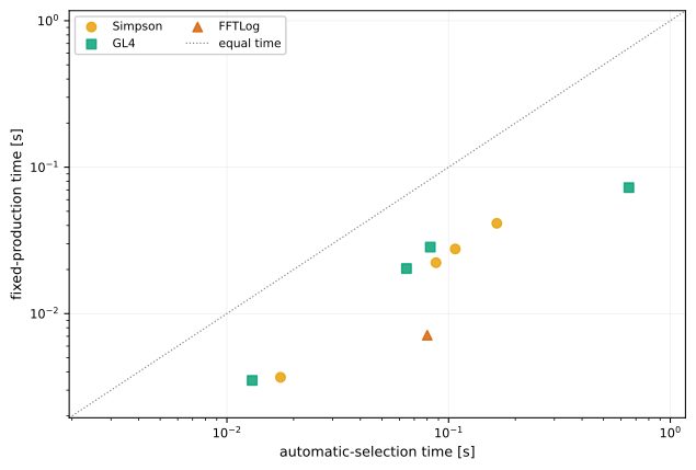
Standard-domain automatic-selection cost at Interaction.rtol = 1e-4. Each marker is one canonical workload with its own automatic-selection time and selected fixed-production time; the dotted diagonal marks equal times. FFTLog [Hamilton, 2000] can have a larger selection-to-production ratio because fixed production is very fast once a stable transform length and bias are known.

Large displacement changes the cost scale:

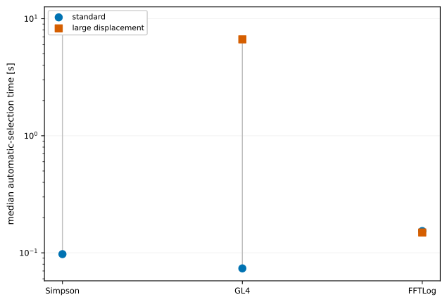
Median automatic-selection time on the canonical matrix in the standard domain (10) and large-displacement domain (11). Large-\(\delta\) finite quadrature must resolve much faster Bessel oscillations and therefore becomes substantially more expensive. FFTLog retains short selection times but automatically accepts only two of four large-domain canonical cases in the declared search box.

Qualified large-displacement production timing

The practical large-displacement benchmark uses Interaction.rtol = 1e-3 over (11). Each point below corresponds to a parameter set that independently passes the reference. Methods without a qualified configuration are omitted.

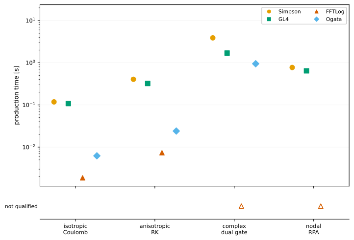
Fixed-production timing for independently qualified large-displacement calculations at Interaction.rtol = 1e-3. The lower status strip uses each method’s color and marker to show method/case combinations for which no independently qualified configuration is present in the tested set; those symbols are status markers, not timing values. The measured times vary strongly with workload and do not define a global method ranking.

The corresponding median production times are generated from the same frozen performance JSON:

Median fixed-production time

Case	Simpson	GL4	FFTLog	Ogata
isotropic Coulomb	0.118 s	0.108 s	0.00187 s	0.00622 s
anisotropic RK	0.405 s	0.323 s	0.00736 s	0.024 s
complex dual gate	3.88 s	1.69 s	not qualified	0.947 s
nodal RPA	0.772 s	0.642 s	not qualified	15.1 s

Qualification source

Case	Simpson	GL4	FFTLog	Ogata
isotropic Coulomb	automatic	automatic	automatic	automatic
anisotropic RK	automatic	automatic	automatic	automatic
complex dual gate	independent	automatic	not qualified	automatic
nodal RPA	independent	automatic	not qualified	independent (terminal)

Some qualified points come from configurations selected automatically. Others use a fixed configuration that passes the independent reference after a conservative automatic refusal. The benchmark JSON records the qualification source explicitly, so automatic selection and independent reference qualification remain distinct.

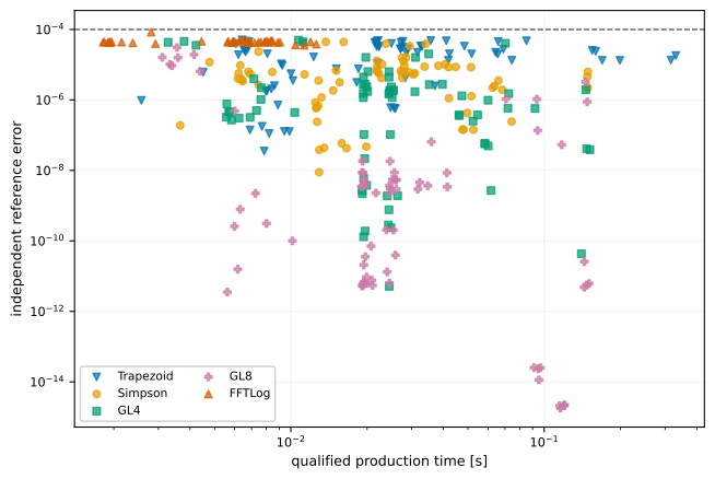
Qualified production timing versus independent-reference error for the broad primary-tolerance matrix. Each marker is one independently qualified case/method calculation, so timing and error belong to the same workload. Method color and marker identify the backend; missing points are combinations that were not independently qualified in this study.

Runtime scaling

For \(N_m\) retained harmonics, \(N_q\) momentum samples, \(N_r\) radial input samples, and effective radial nodes \(N_s\), the leading sampled transform work is

\[ T_H=\Theta(N_mN_qN_s). \]

For Interaction, let \(N_p=N_m^{(1)}N_m^{(2)}\) and let \(N_D\) be the number of displacement vectors. Finite-grid work scales as

\[ T_{\mathrm{finite}}=\Theta(N_pN_DN_{q,s}), \]

and FFTLog as

\[ T_{\mathrm{FFTLog}} =\Theta\!\left[N_p\left(N_F\log N_F+N_D\right)\right]. \]

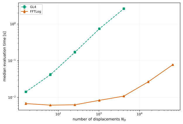
Measured Interaction evaluation time as the requested displacement count \(N_D\) increases with all other benchmark dimensions fixed. Error bars show the timing interquartile range. Finite GL4 approaches the expected linear dependence on \(N_D\). FFTLog pays for a logarithmic transform per harmonic pair and then reuses that representation over the displacement array, so its measured \(N_D\) dependence is much weaker in this regime.

Peak memory

The sampled HarmonicTransform processes q points in batches. With internal batch size \(B\) and \(B_{\mathrm{eff}}=\min(B,N_q)\), the leading model is

\[ M_H=\Theta(N_mN_q+B_{\mathrm{eff}}N_s+N_r). \]

Interaction has

\[ M_{\mathrm{finite}} =\Theta(N_pN_D+N_DN_{q,s}+N_q) \]

and

\[ M_{\mathrm{FFTLog}} =\Theta(N_pN_D+N_F+N_q). \]

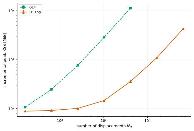
Baseline-subtracted peak resident memory as \(N_D\) increases. Error bars show the interquartile range from fresh-process measurements. The benchmark measures only the incremental Interaction cost above the preconstructed input fields. Both methods retain pair-resolved output arrays proportional to \(N_pN_D\); the finite branch also carries q-quadrature work arrays.

Reproducing the evidence

Tutorial figures are self-contained and can be regenerated from a fresh checkout with

python docs/scripts/generate_figures.py examples

Validation figures and numerical prose require an explicit canonical publication bundle. To refresh both from the same bundle and verify the artifact manifest, run

python docs/scripts/regenerate_publication_evidence.py \
    --results-dir benchmarks/results

This command reads frozen benchmark output. It does not rerun the publication benchmark suite.