User guide

In localized-basis models, the numerical problem begins with a physical interaction tensor: orbital products define the transition fields, the material or electrostatic environment defines the radial kernel, and lattice geometry defines the relative displacements. Direct, exchange, pair-hopping, and correlated-hopping matrix elements differ by those orbital products rather than by separate numerical machinery.

The User Guide follows that calculation: define the four-center matrix element, prepare the two transition fields, transform them, evaluate the radial interaction, inspect the numerical diagnostics, and reuse converged settings when the same numerical problem is evaluated repeatedly.

Four-center matrix elements

Direct, exchange, pair-hopping, correlated-hopping, and general orbital products expressed through the two transition fields used by QUARTIC2D.

Four-center matrix elements

Preparing transition fields

Callable and sampled complex transition fields, PETAL2D representation, reconstruction diagnostics, and plotting helpers.

Preparing transition fields

Momentum-space harmonics

Harmonic transforms, built-in profile plots, q support, diagnostics, calibration, and round-trip checks.

Momentum-space harmonics

Evaluating interactions

Displacement arrays, harmonic-pair contributions, interaction calibration, and method-aware convergence plots.

Evaluating interactions

Convergence and diagnostics

Tolerance semantics, automatic parameter searches, convergence records, failure inspection, and parameter reuse.

Convergence and diagnostics

Choosing numerical methods

Operational guidance for finite rules, FFTLog, and Ogata, with detailed benchmark evidence kept in Validation.

Choosing numerical methods

Outputs and plotting

Built-in plotting helpers, transformed harmonics, interaction arrays, angular-pair contributions, and custom plots.

Outputs and plotting

Performance and reuse

Reuse of transformed fields and calibrated parameters, provenance records, scaling, and repeated calculations.

Performance and reuse

A practical numerical workflow

Most calculations fit one of three levels of numerical control.

Goal	Recommended workflow
inspect a new physical model	construct with defaults, inspect PETAL2D and HarmonicTransform diagnostics, plot the transformed harmonics
report a result with an explicit numerical criterion	call converge_parameters(...), inspect plot_convergence(), then construct the production object from the returned result
evaluate a related family efficiently	calibrate representative difficult members, freeze a justified common parameter envelope, and spot-check the family

The default constructors are intentionally convenient, but they do not silently claim a particular error tolerance. When numerical precision matters, request it explicitly through the appropriate convergence helper.

Representative outputs from the workflow are shown below. The guided examples and the pages linked from this guide explain each stage in full.

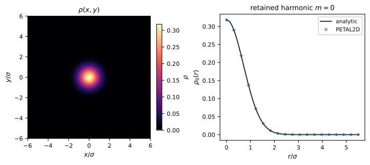
A transition-field representation from PETAL2D.

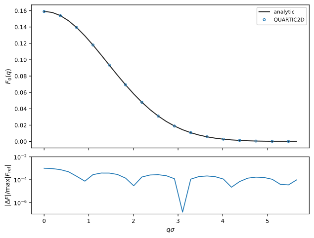
A transformed harmonic together with its independent analytic comparison.

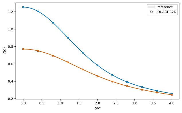
A physical interaction sweep comparing Coulomb and Rytova–Keldysh kernels.

HarmonicTransform.converge_parameters(...) selects momentum support, q-grid resolution, and radial Hankel resolution. Interaction.converge_parameters(...) refines the assembled interaction over the supplied displacement set. Both return public result objects with the same core workflow:

hcal = HarmonicTransform.converge_parameters(
    decomposition,
    rtol=1e-4,
    q_tail_rtol=1e-3,
)
fig, axes = hcal.plot_convergence()
field = hcal.transform(decomposition)
harmonic_record = hcal.to_dict()

ical = Interaction.converge_parameters(
    deltas, field_13, field_42, U_q, rtol=1e-4
)
fig, axes = ical.plot_convergence()
interaction = ical.interaction(deltas, field_13, field_42, U_q)
interaction_record = ical.to_dict()

The calibrated production objects retain the convergence record and expose plot_convergence() themselves. The requested rtol values are self-convergence criteria for represented numerical objects. They are not pointwise error bounds against an unknown exact solution.

Documentation sequence

Start with Getting started for a complete calculation that uses the inspection and convergence helpers directly. Then use Preparing transition fields, Momentum-space harmonics, and Evaluating interactions for the physical and numerical objects themselves.

Convergence and diagnostics explains the tolerance vocabulary and how to inspect a search. Choosing numerical methods gives operational method-selection guidance without duplicating the release benchmark tables. The supporting evidence lives under Validation and benchmarks. Outputs and plotting collects the built-in plotting and inspection API in one place.