Momentum-space harmonics

HarmonicTransform maps every retained PETAL2D radial harmonic to momentum space,

\[ F_m(q)=\int_0^\infty r\,dr\,\rho_m(r)J_m(qr). \]

The input functions \(\rho_m(r)\) come directly from the PETAL2D decomposition in Preparing transition fields.

Construct and inspect a transform

from quartic2d import HarmonicTransform

field = HarmonicTransform(decomposition)

print("method:", field.method)
print("interpolator:", field.interpolator)
print("harmonics:", field.m_values.tolist())
print("q range:", field.q[0], field.q[-1])
print("n_q:", field.q.size)
print("diagnostics healthy:", field.diagnostics.healthy)

The ordinary constructor is useful for exploration. It chooses a scale-aware momentum interval and sampling density from the represented real-space field, then runs inexpensive fault detectors.

The transformed harmonics should normally be inspected directly with the public plotting helper:

fig, axes = field.plot_harmonics()

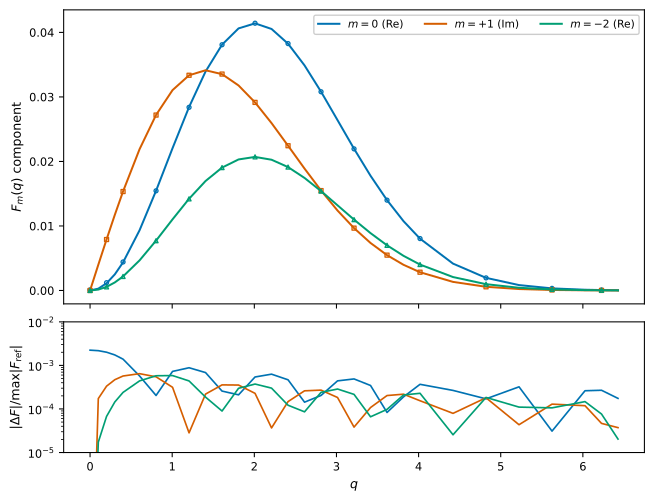
A representative transformed-field plot for a complex transition field.

field.plot() is the compact equivalent when only the transformed profiles are needed:

fig, axes = field.plot()

A stored harmonic can also be evaluated as a function:

import numpy as np

q_eval = np.array([0.0, 1.0, 2.0])
F0 = field(0, q_eval)
print(F0.shape)

(3,)

Fast diagnostics

field.diagnostics.healthy is a fault-detector summary. It does not state that a requested rtol has been satisfied and it is not an independent accuracy estimate.

If the summary is unhealthy, inspect the actual issues:

if not field.diagnostics.healthy:
    print(field.diagnostics.warning_message())
    for issue in field.diagnostics.issues:
        print(issue)

The structured diagnostic record can also be retained with other provenance metadata:

diagnostic_record = field.diagnostics.to_dict()

Typical problems include insufficient represented q support or suspicious behavior near the q boundary. Those warnings are reasons to inspect or refine the representation, not to bypass the checks.

Momentum support and q sampling

q_max is the largest represented momentum. It is part of the numerical representation rather than merely a quadrature option. The PETAL2D radial spacing imposes a radial sampling ceiling,

\[ q_{\mathrm{Nyquist}}=\frac{\pi}{\Delta r}. \]

QUARTIC2D rejects a requested q_max beyond that ceiling. If the physical field requires more momentum support, refine the upstream radial representation.

A fixed interval can be supplied explicitly when the model requires it:

field = HarmonicTransform(
    decomposition,
    q_max=8.0,
    n_q=192,
)

An explicit q_grid is also supported and is used when a calibrated grid is reused in production.

The q-grid interpolation error is distinct from the radial quadrature error used to evaluate each stored \(F_m(q)\) value. Automatic calibration treats these as separate numerical questions.

Radial quadrature

Finite radial rules refine each original radial interval by subdivisions. For example,

field = HarmonicTransform(
    decomposition,
    method="gl4",
    subdivisions=2,
)

simpson, trapezoid, gl4, and gl8 are finite-rule options. Ogata [Ogata, 2005] is an optional specialist radial transform and has its own coupled numerical parameters. Method-selection guidance is in Choosing numerical methods. Detailed performance and validation evidence is kept under Validation and benchmarks.

Automatic calibration

Use converge_parameters(...) when the transformed field needs an explicit self-convergence criterion:

calibration = HarmonicTransform.converge_parameters(
    decomposition,
    rtol=1e-4,
    atol=1e-12,
    q_tail_rtol=1e-3,
    method="simpson",
)

print("converged:", calibration.converged)
print("selected parameters:", calibration.parameters)

The result separates three tasks:

1. selecting sufficient momentum support;

2. resolving interpolation on the stored q grid;

3. refining the radial Hankel quadrature.

The most useful first inspection is the convergence plot:

fig, axes = calibration.plot_convergence()

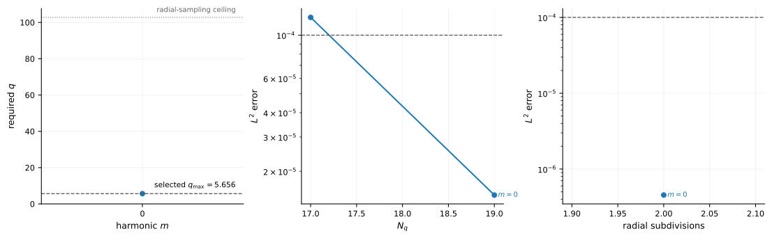
A typical harmonic-transform convergence plot returned by HarmonicTransform.converge_parameters(...).

The three panels display the q-support choice, q-grid refinement, and radial quadrature refinement that produced the selected production parameters. The horizontal criteria in those panels are internal numerical criteria. They are not independent exact-solution error bounds.

Construct a production transform without repeating the search:

field = calibration.transform(decomposition)

The production object carries the same records:

print(field.sampling_convergence is not None)
print(field.quadrature_convergence is not None)
fig, axes = field.plot_convergence()

field.plot(show_convergence=True) is a convenience when both the transformed profiles and the attached convergence record should be displayed:

profiles, convergence = field.plot(show_convergence=True)

The two return values are (fig, axes) pairs for the profile and convergence figures respectively.

Programmatic convergence records

For automated workflows the same information is available without plotting:

sampling = field.sampling_convergence
quadrature = field.quadrature_convergence

The exact structured fields depend on the numerical search, while the public HarmonicConvergenceResult provides the stable high-level interface through converged, parameters, plot_convergence(), transform(), and to_dict().

Store the result when reproducibility matters:

record = calibration.to_dict()

The dictionary is JSON-serializable and contains the selected parameters, tolerances, momentum-support record, and quadrature history.

Round-trip consistency

A transformed field can be mapped numerically back through the corresponding Hankel transform and compared with the represented radial harmonics:

error = field.roundtrip_error()
print(f"round-trip relative L2: {error:.3e}")

This is a useful forward/inverse consistency diagnostic. It is not an independent error estimate for the original continuum orbital or transition field because both directions operate on the same represented numerical data.

What rtol means

For ordered refinement, HarmonicTransform.rtol controls the relative \(L^2\) change between successive represented transforms. Acceptance also requires the peak-scaled absolute maximum-change condition controlled by atol. q_tail_rtol separately controls the estimated omitted q-space norm beyond the selected q_max.

The precise criteria, failure interpretation, and relationship to independent validation are developed in Convergence and diagnostics.