Evaluating interactions#

After both transition fields have been transformed, Interaction assembles the four-center matrix element over the requested displacement vectors.

from quartic2d import Interaction

interaction = Interaction(
    deltas,
    field_13,
    field_42,
    U_q,
)

print("method:", interaction.method)
print("number of displacements:", interaction.V.size)

The ordinary constructor is intended for exploratory evaluation. The default method is GL4. When a numerical tolerance matters, calibrate the target fields, kernel, and displacement domain explicitly rather than treating a constructor default as an accuracy statement.

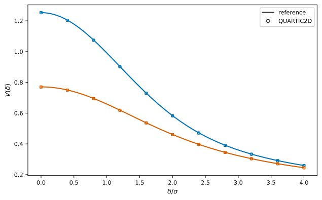
Coulomb and Rytova-Keldysh interactions between localized Gaussian states — A representative interaction output: the same localized state evaluated with two radial kernels.#

Returned arrays#

For \(N_m^{(1)}\) harmonics in the first transformed field, \(N_m^{(2)}\) in the second, and \(N_D\) displacements, the principal arrays have shapes

Phi_mm : (N_m1, N_m2, N_D)
H_mm   : (N_m1, N_m2, N_D)
V_mm   : (N_m1, N_m2, N_D)
V      : (N_D,)

Inspect the actual calculation directly:

print(interaction.Phi_mm.shape)
print(interaction.H_mm.shape)
print(interaction.V_mm.shape)
print(interaction.V.shape)

The total matrix element is

\[ U_{1234}(\boldsymbol\delta) =\sum_{m,m'}U_{1234}^{(m,m')}(\boldsymbol\delta), \]

represented by interaction.V. V_mm keeps the angular-pair decomposition. H_mm contains the radial integrals before the displacement-dependent angular prefactors in Phi_mm are applied.

Displacement geometry#

For anisotropic transition fields, both the magnitude and direction of \(\boldsymbol\delta\) can matter. A fixed-radius angular sweep is

import numpy as np

radius = 2.0
phi_delta = np.linspace(0.0, 2.0 * np.pi, 181)
deltas = np.column_stack(
    (radius * np.cos(phi_delta), radius * np.sin(phi_delta))
)

interaction = Interaction(deltas, field_13, field_42, U_q)

The returned values preserve the displacement ordering. A complete anisotropic example is given in Orientation-dependent interactions of anisotropic localized states.

Complex matrix elements#

V and V_mm are complex arrays. A real result occurs only when the supplied transition fields, kernel, geometry, and orbital conventions imply it. Exchange, pair-hopping, correlated-hopping, and other off-diagonal four-center channels need not be positive or purely real.

Do not discard an imaginary component simply because a density-density example was real. If Hermiticity, point-group symmetry, or orbital conventions predict a relation among index permutations, use that relation as a physical consistency check.

Automatic interaction calibration#

Interaction.converge_parameters(...) refines the assembled interaction over the supplied displacement set:

calibration = Interaction.converge_parameters(
    deltas,
    field_13,
    field_42,
    U_q,
    rtol=1e-4,
    atol=1e-12,
    method="gl4",
)

print("converged:", calibration.converged)
print("method:", calibration.method)
print("selected parameters:", calibration.parameters)

The displacement set is part of the numerical problem. If production extends to substantially larger separations or introduces a different angular domain, that change must be covered by the calibration or justified separately.

Inspect the search#

The public convergence result has a method-aware plotting helper:

fig, axes = calibration.plot_convergence()

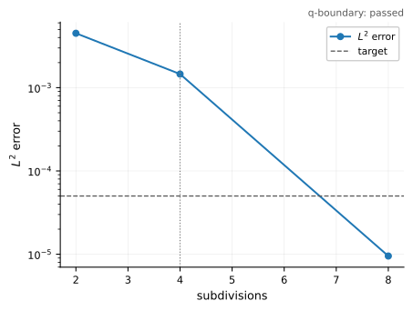
A typical interaction convergence plot returned by Interaction.converge_parameters(...).#

For finite rules, the panels show refinement changes and the observed asymptotic order. FFTLog displays its resolution and bias-robustness search. Ogata displays the coupled \((N,h)\) refinement. These plots visualize the internal search used to select parameters. They do not show an independent reference error.

Build and inspect the production interaction#

Construct the production object from the selected settings without rerunning the search:

interaction = calibration.interaction(
    deltas,
    field_13,
    field_42,
    U_q,
)

The production object carries the result through its public convergence attribute:

print(interaction.convergence is calibration)
fig, axes = interaction.plot_convergence()

True

The result can be serialized for provenance:

record = calibration.to_dict()

By default the record omits the full interaction arrays stored during the search. Use calibration.to_dict(include_values=True) only when retaining those arrays is actually useful.

Reusing a calibration#

The selected parameters can be reused only when the numerical problem remains appropriately represented by the calibration. Reuse is straightforward for an identical field pair, kernel, and displacement domain:

params = calibration.parameters
repeat = Interaction(deltas, field_13, field_42, U_q, **params)

calibration.interaction(...) is preferable when the convergence record should stay attached to the production object.

For a family of related kernels or fields, define and validate a common parameter envelope from representative difficult members rather than copying a single-point calibration blindly. The family strategy is discussed in Calibrate families, not every point.

Choosing a numerical method#

Finite rules, FFTLog, and Ogata have different refinement structures. The operational distinctions are summarized in Choosing numerical methods. Detailed benchmark coverage and performance belong in Validation and benchmarks.