Orientation-dependent interactions of anisotropic localized states#

Localized states in low-symmetry two-dimensional materials, anisotropic quantum dots, and Wannier bases need not be rotationally symmetric. Their interaction can therefore depend on the direction connecting two centers, so a scalar distance alone is insufficient to characterize the matrix element.

An anisotropic transition field generates this orientation dependence directly. Consider

\[ \rho(r,\theta) = \frac{e^{-r^2}}{\pi} \left[1+a r^2\cos(2\theta)\right], \qquad a=0.35. \]

The exact angular content is \(m=0,\pm2\). The corresponding transforms are

\[ F_0(q)=\frac{e^{-q^2/4}}{2\pi}, \qquad F_{\pm2}(q)=\frac{a q^2}{16\pi}e^{-q^2/4}. \]

Decompose and calibrate#

dec = make_decomposition()
hcal = HarmonicTransform.converge_parameters(
    dec,
    rtol=1.0e-4,
    atol=1.0e-12,
    q_tail_rtol=1.0e-3,
    method="simpson",
    verbose=False,
)
field = hcal.transform(dec)

hcal.plot_convergence()
field.plot_harmonics()

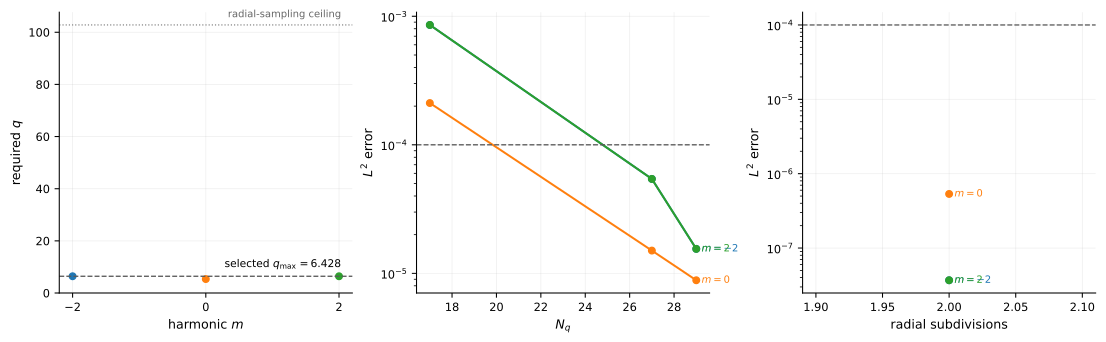
Harmonic-transform self-convergence diagnostics for the anisotropic transition field — Self-convergence diagnostics for the anisotropic harmonic transform.#

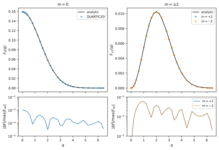
Harmonic Hankel transforms of the anisotropic transition field — The \(m=0\) and \(|m|=2\) components are transformed independently. Solid curves show the analytic Hankel transforms of these components and open markers show the corresponding QUARTIC2D values.#

Resolve the angular dependence#

For \(m,m'\in\{0,\pm2\}\), the interaction contains only angular differences \(0\), \(\pm2\), and \(\pm4\). For a real field these combine into

\[ V(\delta,\varphi_\delta) = A_0(\delta) +A_2(\delta)\cos 2\varphi_\delta +A_4(\delta)\cos 4\varphi_\delta. \]

The interaction is calibrated on the complete angular scan before the production values are evaluated:

ical = Interaction.converge_parameters(
    vectors,
    field,
    field,
    yukawa,
    rtol=1.0e-4,
    atol=1.0e-12,
    method="gl4",
    verbose=False,
)
interaction = ical.interaction(vectors, field, field, yukawa)
ical.plot_convergence()

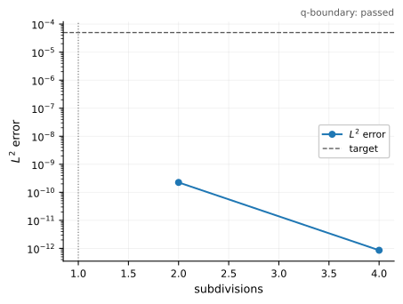
Interaction self-convergence diagnostics for the anisotropic interaction — Self-convergence diagnostics for the anisotropic interaction calibration.#

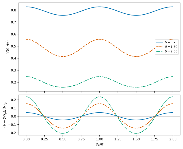
Orientation dependence of the anisotropic interaction at three separations — The upper plot shows the interaction versus displacement angle at three separations. The lower plot shows the fractional angular modulation relative to each curve’s angular mean. The anisotropy is strongest when the localized states substantially overlap and decreases with separation.#

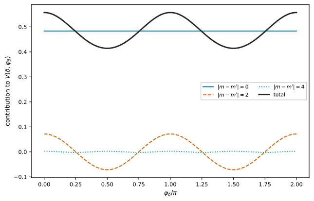
Harmonic-pair contributions to the anisotropic interaction — Grouping the returned `V_mm` array by \(|m-m'|\) isolates the isotropic, twofold, and fourfold contributions at \(\delta=1.5\). The black curve is their sum and reproduces the full interaction to floating-point precision.#

PETAL2D
retained harmonics: [0, 2, -2]
m=+0: power fraction=0.970276
m=+2: power fraction=0.014862
m=-2: power fraction=0.014862
PETAL2D target reached: True

HarmonicTransform
harmonic transform converged: True
harmonic quadrature: simpson
retained harmonics: [0, 2, -2]
F_0(0) = 0.15915476

Interaction
interaction converged: True
interaction quadrature: gl4
delta=0.75: V(0)=0.827885, V(pi/2)=0.756552
delta=1.50: V(0)=0.557855, V(pi/2)=0.414590
delta=2.50: V(0)=0.247386, V(pi/2)=0.158939
harmonic-pair reconstruction relative max residual: 7.961e-16

The complete calculation is examples/anisotropic_interaction.py.