Sampled transition fields on a Cartesian grid

Electronic-structure and continuum calculations usually provide localized states numerically rather than as closed-form functions. Wannier functions, defect states, quantum-dot eigenstates, and continuum-model wavefunctions may therefore enter an interaction calculation as values on a Cartesian grid.

QUARTIC2D does not require analytic input functions. To represent that workflow while keeping an exact reference available, sample the normalized states

\[ \phi_s=\frac{e^{-r^2/2}}{\sqrt\pi}, \qquad \phi_+=\frac{x+iy}{\sqrt\pi}e^{-r^2/2}. \]

The forward transition field is

\[ \rho_{s+}=\phi_s^*\phi_+ =\frac{r e^{-r^2}}{\pi}e^{i\theta}, \]

so only \(m=+1\) is present. The reverse field contains only \(m=-1\).

Supply arrays to PETAL2D

X, Y = np.meshgrid(x, y, indexing="ij")
r2 = X**2 + Y**2
psi_s = np.exp(-0.5 * r2) / np.sqrt(np.pi)
psi_p_plus = (X + 1j * Y) * np.exp(-0.5 * r2) / np.sqrt(np.pi)

rho_forward = np.conj(psi_s) * psi_p_plus
rho_reverse = np.conj(psi_p_plus) * psi_s

dec_forward = PolarDecomposition(
    rho_forward,
    x,
    y,
    Nr=181,
    Ntheta=256,
    rmax=5.5,
    origin=(0.0, 0.0),
    interp_method="cubic",
    recon_err_tol=1.0e-2,
)

recon_err_tol is expressed in percent.

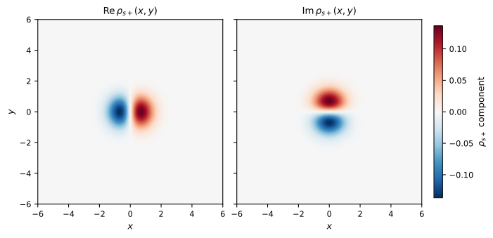
Cartesian samples of the complex transition field. Both panels use the same color normalization so the real and imaginary components can be compared directly.

Transform and inspect the sampled harmonic

The exact forward transform is

\[ F_1(q)=\frac{q}{4\pi}e^{-q^2/4}. \]

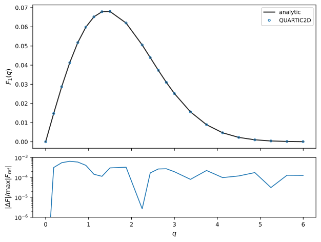
The transformed retained harmonic compared with the analytic result. The lower panel is an independent pointwise comparison normalized by the peak analytic transform; it is separate from the automatic self-convergence criteria.

hcal = HarmonicTransform.converge_parameters(
    dec_forward,
    rtol=1.0e-4,
    atol=1.0e-12,
    q_tail_rtol=1.0e-3,
    method="simpson",
    verbose=False,
)
field_forward = hcal.transform(dec_forward)
hcal.plot_convergence()

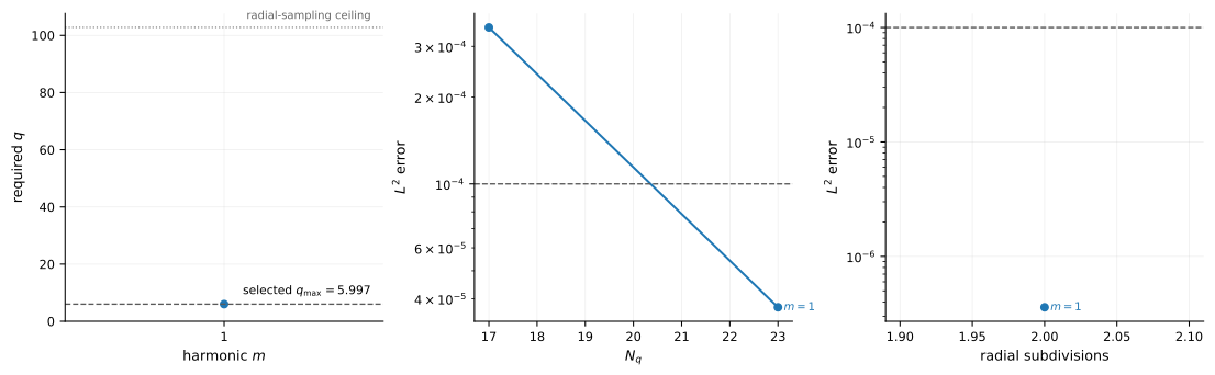
Self-convergence diagnostics for the sampled-data harmonic transform.

The analytic errors reported below can exceed rtol=1e-4 because rtol compares successive QUARTIC2D calculations, whereas the analytic comparison also includes the upstream Cartesian-to-polar representation error.

Continue to a four-center interaction

The sampled-data path is otherwise identical to the callable-field path. After calibrating both forward and reverse transforms, evaluate an off-diagonal Yukawa-screened interaction:

ical = Interaction.converge_parameters(
    calibration_vectors,
    field_forward,
    field_reverse,
    yukawa,
    rtol=1.0e-4,
    atol=1.0e-12,
    method="gl4",
    verbose=False,
)
interaction = ical.interaction(
    vectors,
    field_forward,
    field_reverse,
    yukawa,
)
ical.plot_convergence()

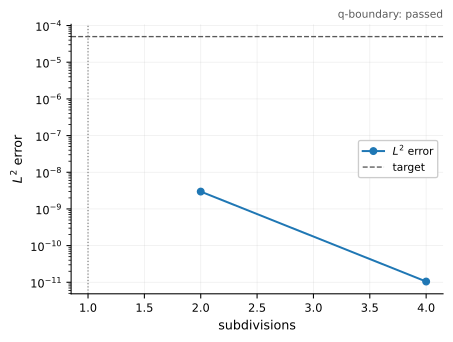
Self-convergence diagnostics for the sampled-data interaction calibration.

The small imaginary parts are numerical roundoff for this symmetry-related forward/reverse pair. The complete executable calculation is examples/sampled_data.py.

Sampled PETAL2D input
array shape: (181, 181)
forward: modes=[1], reconstruction error=6.250e-05%, domain consistency=0.99999906
reverse: modes=[-1], reconstruction error=6.250e-05%, domain consistency=0.99999906

HarmonicTransform
all self-convergence criteria satisfied: True
forward analytic relative L2 error: 5.093e-04
forward peak-normalized max error: 6.477e-04

Interaction
self-convergence satisfied: True
delta=0.0  V=+0.000000+0.00e+00j
delta=1.0  V=-0.074457+1.85e-17j
delta=2.0  V=-0.089729+2.23e-17j
delta=4.0  V=-0.010301+2.57e-18j