Dielectric screening of multiorbital interaction channels#

In two-dimensional materials, substrate choice, encapsulation, nearby gates, and dielectric engineering can modify the effective interaction without changing the underlying localized orbitals. Parameter studies therefore often require the same orbital matrix elements over a family of screening lengths or dielectric environments.

The complex-orbital fields from Complex localized orbitals and off-diagonal Coulomb matrix elements are retained while only the radial interaction kernel changes. Once the transition fields have been transformed, a family of radial kernels can be evaluated without repeating the PETAL2D decomposition.

For Rytova–Keldysh screening [Keldysh, 1979, Rytova, 1967],

\[ U(q;r_0)=\frac{2\pi}{q(1+r_0q)}. \]

We vary \(r_0\) while keeping the three channels

exchange,
pair hopping,
correlated hopping

fixed.

Calibrate a bounded kernel family#

A production sweep should not silently assume that one kernel calibration is valid for every parameter value. The example therefore calibrates representative screening lengths

\[ r_0=0.1,\ 1,\ 10 \]

for each channel and takes the most refined finite-rule setting found within that bounded family.

representative_r0 = (0.1, 1.0, 10.0)

calibrations = {
    (name, r0): Interaction.converge_parameters(
        calibration_vectors,
        first,
        second,
        rytova_keldysh(r0),
        rtol=1.0e-4,
        atol=1.0e-12,
        method="gl4",
        verbose=False,
    )
    for name, (first, second) in channels.items()
    for r0 in representative_r0
}

# Inspect one representative search directly.
calibrations[("exchange", 1.0)].plot_convergence()

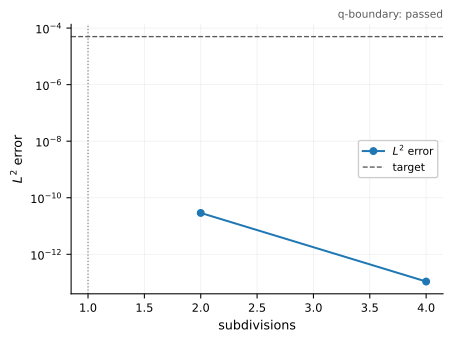
Interaction self-convergence diagnostics for a representative screened exchange channel — Self-convergence diagnostics for the representative \(r_0=1\) exchange calibration.#

This is a family-specific reuse decision, not a universal statement about all Rytova–Keldysh parameters or all transition fields.

Reuse the calibrated resolution#

The public example uses a modest \(31\times41\) screening/displacement grid so it remains suitable as a tutorial rather than a benchmark workload:

r0_values = np.geomspace(0.1, 10.0, 31)
delta = np.linspace(0.0, 4.0, 41)

It evaluates three interaction channels, for 3813 matrix elements in total.

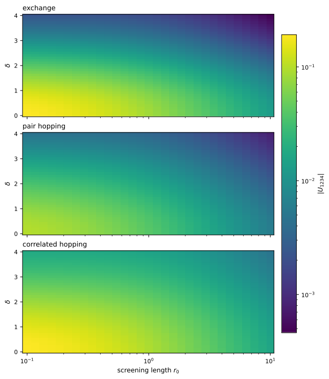
Screening-length and displacement dependence of three multiorbital interaction channels on a shared magnitude scale — Magnitude of the exchange, pair-hopping, and correlated-hopping channels versus screening length and displacement. All three plots use the same logarithmic color normalization, so color has the same quantitative meaning for every channel. The figure visualizes parameter reuse across the bounded screening family.#

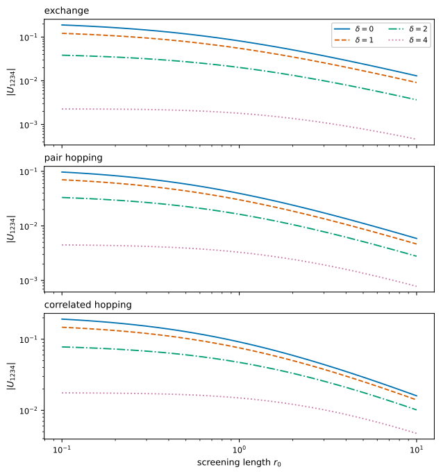
Representative screening-length cuts of the multiorbital interaction channels — Representative cuts at \(\delta=0,1,2,\) and \(4\) show how the magnitude of each interaction channel changes with screening length. The same displacement styles are used in all three plots.#

Calibration
all harmonic searches satisfied: True
all representative interaction searches satisfied: True
representative screening lengths: (0.1, 1.0, 10.0)
common GL4 subdivisions: 1

Production sweep
screening lengths: 31
displacements: 41
channels: 3
matrix elements evaluated: 3813
exchange           V(delta=2,r0=0.1)=-0.00034-0.03847j  V(delta=2,r0=10)=+0.00115-0.00349j
pair hopping       V(delta=2,r0=0.1)=+0.03318+0.00000j  V(delta=2,r0=10)=+0.00278+0.00000j
correlated hopping V(delta=2,r0=0.1)=+0.02298+0.07449j  V(delta=2,r0=10)=+0.00420+0.00923j

The complete calculation is examples/screening_family_sweep.py. The larger publication stress sweeps remain under benchmarks/ and are intentionally not part of this guided example.