Localized-state interactions in a 2D dielectric environment#

In two-dimensional semiconductors and other atomically thin systems, the interaction between localized carriers depends strongly on dielectric screening by the layer and its surroundings. Effective lattice models therefore need matrix elements for both the localized states and the appropriate screened kernel, rather than a single geometry-independent Coulomb parameter.

A normalized localized state provides a complete PETAL2D → QUARTIC2D calculation with analytic formulas for both the transformed field and the interaction.

With lengths measured in units of the Gaussian width,

\[ \rho(r)=\frac{e^{-r^2}}{\pi}, \qquad F_0(q)=\frac{e^{-q^2/4}}{2\pi}. \]

Rotational symmetry leaves only \(m=0\). The calculation compares the bare Coulomb kernel

\[ U_{\rm C}(q)=\frac{2\pi}{q} \]

with a Rytova–Keldysh kernel [Keldysh, 1979, Rytova, 1967]

\[ U_{\rm RK}(q)=\frac{2\pi}{q(1+r_0q)}, \qquad r_0=1. \]

Decompose and inspect the field#

import numpy as np
from petal2d import PolarDecomposition
from quartic2d import HarmonicTransform, Interaction

x = np.linspace(-6.0, 6.0, 181)
y = np.linspace(-6.0, 6.0, 181)


def density(x, y):
    return np.exp(-(x**2 + y**2)) / np.pi


dec = PolarDecomposition(
    density,
    x,
    y,
    Nr=181,
    Ntheta=256,
    rmax=5.5,
    origin=(0.0, 0.0),
    recon_err_tol=1.0e-10,
)

print("retained modes:", dec.m_sorted)
print(f"reconstruction error [%]: {dec.recon_error_measured:.3e}")
print(f"domain consistency: {dec.domain_consistency:.8f}")

PETAL2D also exposes plotting helpers for inspecting the retained angular content and the reconstruction:

dec.plot_harmonics_with_hist("Gaussian angular decomposition")
dec.plot_original_vs_reconstructions("Gaussian reconstruction")

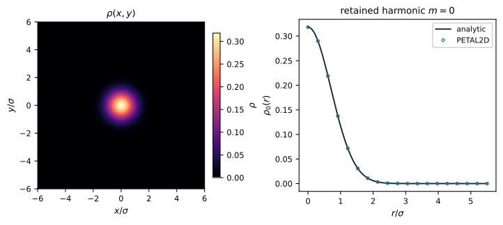
PETAL2D decomposition of a normalized isotropic Gaussian — The isotropic Gaussian is represented entirely by the \(m=0\) channel. The reconstruction and spectral-power diagnostics concern the PETAL2D representation of the input field, not the downstream Hankel-transform error.#

Calibrate the harmonic transform#

hcal = HarmonicTransform.converge_parameters(
    dec,
    rtol=1.0e-4,
    atol=1.0e-12,
    q_tail_rtol=1.0e-3,
    method="simpson",
    verbose=False,
)
field = hcal.transform(dec)

exact = np.exp(-field.q**2 / 4.0) / (2.0 * np.pi)
relative_l2 = (
    np.linalg.norm(field.F_q[0].real - exact)
    / np.linalg.norm(exact)
)

print("self-convergence satisfied:", hcal.converged)
print(f"analytic relative L2 error: {relative_l2:.3e}")

The convergence record is directly inspectable:

hcal.plot_convergence()
field.plot_harmonics()

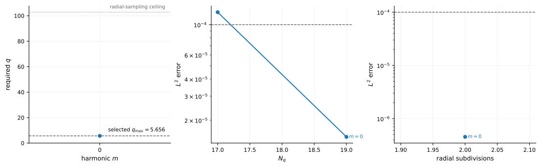
Harmonic-transform self-convergence diagnostics for the isotropic Gaussian example — Self-convergence diagnostics used to select the harmonic-transform parameters.#

The requested rtol=1e-4 controls refinement changes inside the automatic search. The analytic error above is a different quantity and need not equal rtol.

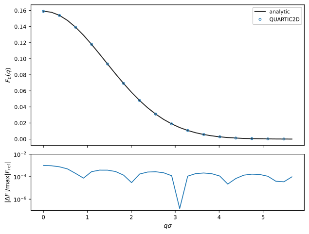
Numerical and analytic harmonic Hankel transform of the Gaussian — The numerical transform is compared with the analytic \(F_0(q)\). The lower reference-error curve is independent of the self-convergence criterion used to select the transform parameters.#

Calibrate and evaluate the interaction#

The transform can now be reused while the interaction quadrature is calibrated on a displacement interval that contains the production domain.

def coulomb(q):
    return 2.0 * np.pi / q


def rytova_keldysh(q, r0=1.0):
    return 2.0 * np.pi / (q * (1.0 + r0 * q))


calibration_delta = np.geomspace(1.0e-2, 1.0e2, 32)
calibration_vectors = np.column_stack(
    (calibration_delta, np.zeros_like(calibration_delta))
)

ccal = Interaction.converge_parameters(
    calibration_vectors,
    field,
    field,
    coulomb,
    rtol=1.0e-4,
    atol=1.0e-12,
    method="gl4",
    verbose=False,
)
rkcal = Interaction.converge_parameters(
    calibration_vectors,
    field,
    field,
    rytova_keldysh,
    rtol=1.0e-4,
    atol=1.0e-12,
    method="gl4",
    verbose=False,
)

# The Interaction calibration has the same inspection workflow.
ccal.plot_convergence()


delta = np.linspace(0.0, 4.0, 81)
vectors = np.column_stack((delta, np.zeros_like(delta)))
bare = ccal.interaction(vectors, field, field, coulomb)
rk = rkcal.interaction(vectors, field, field, rytova_keldysh)

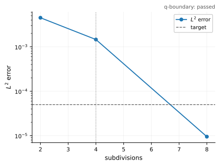
Interaction self-convergence diagnostics for the isotropic Gaussian example — Self-convergence diagnostics for the Coulomb interaction calibration.#

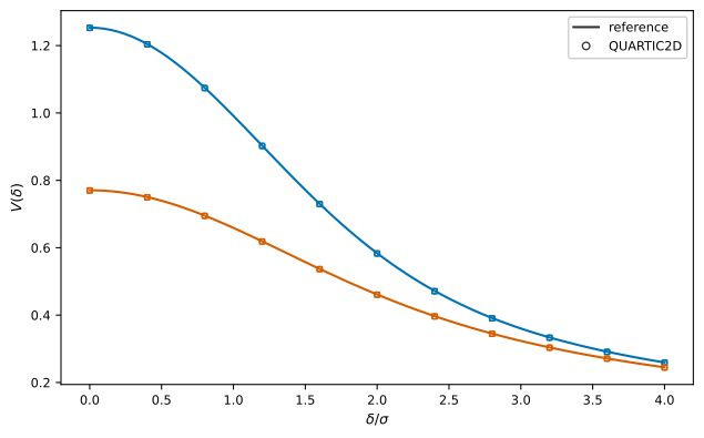
Coulomb and Rytova-Keldysh interactions between localized Gaussian states — Interaction versus displacement for the same localized field. Blue denotes the Coulomb kernel and orange denotes the Rytova–Keldysh kernel. Solid curves show the analytic matrix elements, open circles show the default QUARTIC2D calculation, and open squares show the self-converged QUARTIC2D calculation. Screening changes the short-distance matrix element most strongly, while the kernels approach the same long-wavelength behavior at large separation.#

PETAL2D
retained modes: [0]
reconstruction error [%]: 1.176e-14
domain consistency: 0.99968873

HarmonicTransform
self-convergence satisfied: True
analytic relative L2 error: 7.486e-04
selected q_max: 5.655935
selected n_q: 19

Interaction
Coulomb self-convergence satisfied: True
Rytova-Keldysh self-convergence satisfied: True
delta=0.0  Coulomb=1.252579  RK=0.769954
delta=1.0  Coulomb=0.990611  RK=0.658185
delta=2.0  Coulomb=0.582827  RK=0.460529
delta=4.0  Coulomb=0.258812  RK=0.244462

The complete executable calculation is examples/isotropic_interaction.py. The PETAL2D representation, harmonic-transform convergence, interaction convergence, and analytic comparison are reported separately.