Complex localized orbitals and off-diagonal Coulomb matrix elements#

Valley, angular-momentum, magnetic, and other phase-carrying orbital bases naturally produce complex transition fields. The corresponding off-diagonal interaction matrix elements cannot be reduced to products of positive real densities; their relative phases are part of the four-center integral.

The orbitals

\[ \phi_s=\frac{e^{-r^2/2}}{\sqrt\pi} \]

and

\[ \phi_h= \frac{e^{-r^2/2}}{2\sqrt\pi} \left[ \sqrt2(1-r^2) +i r e^{i\theta} +\frac{r^2}{\sqrt2}e^{-2i\theta} \right]. \]

The transition field \(\rho_{sh}=\phi_s^*\phi_h\) contains exactly \(m=0,+1,-2\), while \(\rho_{hs}=\rho_{sh}^*\) contains \(m=0,-1,+2\).

Transform the complex channels#

The analytic transforms are

\[ F_{sh,0}=\frac{q^2}{8\sqrt2\pi}e^{-q^2/4}, \qquad F_{sh,1}=\frac{i q}{8\pi}e^{-q^2/4}, \qquad F_{sh,-2}=\frac{q^2}{16\sqrt2\pi}e^{-q^2/4}. \]

The \(ss\), \(sh\), and \(hs\) transforms are converged independently.

Those are independent analytic errors, not the internal self-convergence quantity. The selected transform can be inspected directly:

hcal["sh"].plot_convergence()
fields["sh"].plot_harmonics()

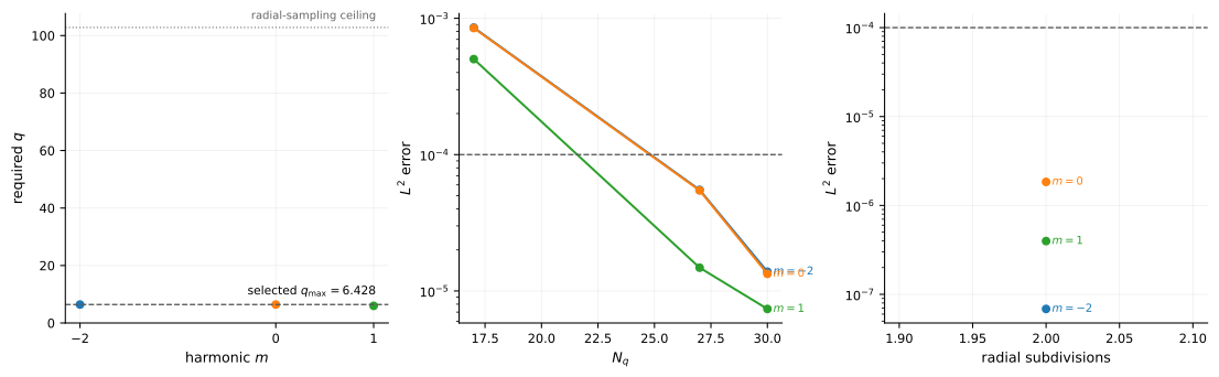
Harmonic-transform self-convergence diagnostics for the complex transition field — Self-convergence diagnostics for the \(sh\) harmonic transform.#

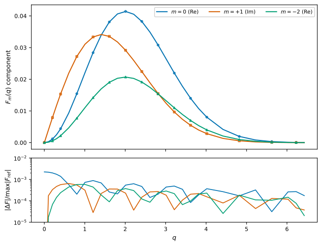
Harmonic transforms of a complex mixed-angular transition field — The three retained angular channels are transformed separately. Solid curves show the analytic components and open markers show QUARTIC2D values; the lower panel gives the independent peak-normalized transform error.#

Build exchange, pair-hopping, and correlated-hopping channels#

Using a dual-gate kernel,

\[ U(q)=\frac{2\pi}{q}\tanh(qd), \]

three representative off-diagonal channels are

channels = {
    "exchange": (fields["sh"], fields["sh"]),
    "pair hopping": (fields["sh"], fields["hs"]),
    "correlated hopping": (fields["ss"], fields["hs"]),
}

ical = {
    name: Interaction.converge_parameters(
        calibration_vectors,
        first,
        second,
        dual_gate,
        rtol=1.0e-4,
        atol=1.0e-12,
        method="gl4",
        verbose=False,
    )
    for name, (first, second) in channels.items()
}

ical["exchange"].plot_convergence()

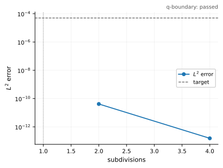
Interaction self-convergence diagnostics for the exchange channel — Self-convergence diagnostics for the exchange interaction calibration.#

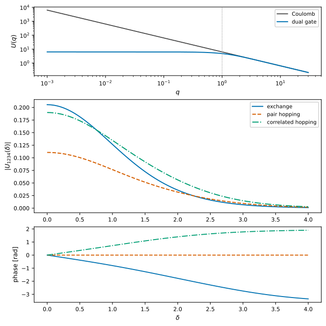
Complex off-diagonal interaction channels under dual-gate screening — The top plot compares the bare Coulomb and dual-gate kernels. The remaining plots show the magnitude and unwrapped phase of the exchange, pair-hopping, and correlated-hopping matrix elements. Complex transition fields enter the same four-center harmonic representation as real transition fields.#

PETAL2D
rho_ss: modes=[0], reconstruction error=1.377e-14%
rho_sh: modes=[0, 1, -2], reconstruction error=2.817e-14%
rho_hs: modes=[0, -1, 2], reconstruction error=2.895e-14%

HarmonicTransform
all self-convergence criteria satisfied: True
m=+0 analytic peak-normalized max error: 2.237e-03
m=+1 analytic peak-normalized max error: 6.462e-04
m=-2 analytic peak-normalized max error: 5.839e-04

Interaction
all self-convergence criteria satisfied: True
delta=0.0
  exchange           +0.20551-0.00000j
  pair hopping       +0.11068-0.00000j
  correlated hopping +0.18999-0.00000j
delta=1.0
  exchange           +0.08785-0.09124j
  pair hopping       +0.07657+0.00000j
  correlated hopping +0.10082+0.08932j
delta=2.0
  exchange           -0.00747-0.03511j
  pair hopping       +0.03194+0.00000j
  correlated hopping +0.00974+0.05535j

The complete script is examples/complex_transition_field.py.