Getting started#

Effective models of localized electrons in two-dimensional materials require interaction parameters obtained by integrating the spatial structure of the localized states against the dielectric interaction. Even the direct interaction between two identical localized states changes when the bare Coulomb kernel is replaced by the screened interaction appropriate to a 2D layer and its environment.

QUARTIC2D evaluates these four-center matrix elements from two transition fields and a radial interaction kernel. The direct interaction of a normalized Gaussian orbital provides an analytic starting point,

\[ \phi(r)=\frac{e^{-r^2/2}}{\sqrt{\pi}}, \qquad \rho(r)=|\phi(r)|^2=\frac{e^{-r^2}}{\pi}, \]

whose only angular harmonic and Hankel transform are

\[ \rho_0(r)=\rho(r), \qquad F_0(q)=\int_0^\infty r\,dr\,\rho_0(r)J_0(qr) =\frac{e^{-q^2/4}}{2\pi}. \]

The bare Coulomb and Rytova–Keldysh kernels [Keldysh, 1979, Rytova, 1967] used below are

\[ U_{\mathrm C}(q)=\frac{2\pi}{q}, \qquad U_{\mathrm{RK}}(q)=\frac{2\pi}{q(1+r_0q)}, \qquad r_0=1. \]

Lengths are measured in units of the Gaussian width and the Coulomb prefactor \(e^2/\epsilon\) is set to unity.

Installation#

python -m pip install quartic2d

The optional Ogata quadrature backend [Ogata, 2005] is installed with

python -m pip install "quartic2d[ogata]"

import quartic2d
print(quartic2d.__version__)

0.1.0

1. Represent the transition field with PETAL2D#

PETAL2D expands the transition field as

\[ \rho(r,\theta)=\sum_m\rho_m(r)e^{im\theta}. \]

import numpy as np
from petal2d import PolarDecomposition
from quartic2d import HarmonicTransform, Interaction

x = np.linspace(-6.0, 6.0, 181)
y = np.linspace(-6.0, 6.0, 181)


def density(x, y):
    return np.exp(-(x**2 + y**2)) / np.pi


dec = PolarDecomposition(
    density,
    x,
    y,
    Nr=181,
    Ntheta=256,
    rmax=5.5,
    origin=(0.0, 0.0),
    recon_err_tol=1.0e-10,
)

print("selected pairs:", dec.selected_pairs)
print("retained modes:", dec.m_sorted)
print(f"measured reconstruction error [%]: {dec.recon_error_measured:.3e}")
print(f"domain consistency: {dec.domain_consistency:.8f}")

Rotational symmetry leaves only \(m=0\). Before transforming a new field, inspect what PETAL2D actually retained rather than assuming the angular content. Its built-in helper gives the radial profiles and retained power fractions directly:

fig, axes = dec.plot_harmonics_with_hist(
    title="Gaussian transition field"
)

For sampled or more complicated fields, also inspect PETAL2D’s reconstruction and domain diagnostics before asking QUARTIC2D to refine the downstream momentum-space calculation. See Preparing transition fields.

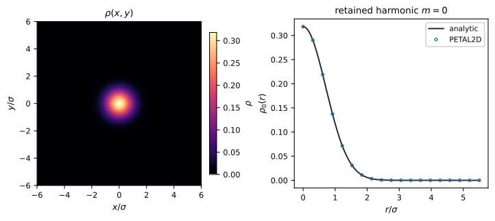
PETAL2D decomposition of a normalized isotropic Gaussian — Normalized Gaussian field and its retained radial harmonic. The analytic radial profile and PETAL2D samples coincide; only \(m=0\) is required for this isotropic transition field.#

2. Transform the retained harmonics#

HarmonicTransform evaluates

\[ F_m(q)=\int_0^\infty r\,dr\,\rho_m(r)J_m(qr) \]

for every retained PETAL2D harmonic.

field = HarmonicTransform(dec)

print("retained harmonics:", field.m_values.tolist())
print("Hankel quadrature:", field.method)
print("diagnostics healthy:", field.diagnostics.healthy)

The transformed profiles are available through a public plotting helper:

fig, axes = field.plot_harmonics()

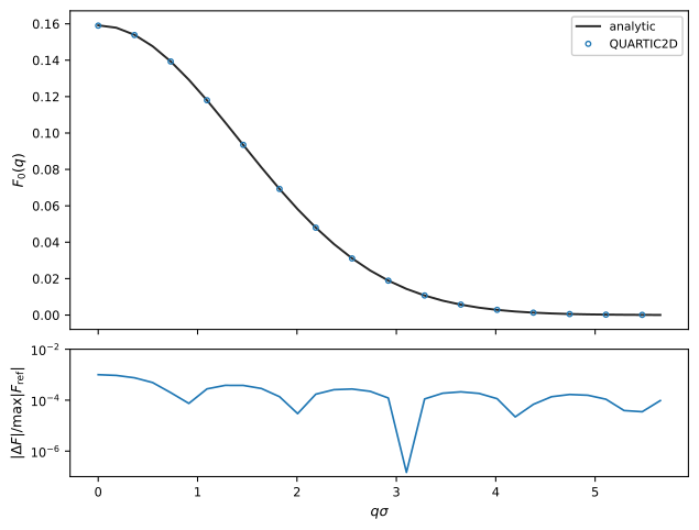
Analytic and numerical Gaussian harmonic Hankel transform with lower error panel — The transformed \(m=0\) harmonic for the Gaussian example. The lower panel is an independent pointwise absolute error normalized by the peak analytic transform.#

or, equivalently for the ordinary profile view,

fig, axes = field.plot()

The fast diagnostics are fault detectors, not an independent accuracy guarantee. If a new input is unhealthy, inspect the reported issues rather than only the Boolean:

if not field.diagnostics.healthy:
    print(field.diagnostics.warning_message())
    for issue in field.diagnostics.issues:
        print(issue)

Because this Gaussian has an analytic transform, an independent error can also be evaluated explicitly:

q = field.q
F0_exact = np.exp(-q**2 / 4.0) / (2.0 * np.pi)
relative_l2 = (
    np.linalg.norm(field.F_q[0].real - F0_exact)
    / np.linalg.norm(F0_exact)
)
print(f"independent analytic relative L2: {relative_l2:.3e}")

That independent error is conceptually different from the self-convergence criteria used below.

3. Evaluate the interaction#

For this isotropic problem,

\[ U(\delta)=2\pi\int_0^\infty q\,dq\, U(q)|F_0(q)|^2J_0(q\delta). \]

def coulomb(q):
    return 2.0 * np.pi / q


def rytova_keldysh(q, r0=1.0):
    return 2.0 * np.pi / (q * (1.0 + r0 * q))


delta = np.linspace(0.0, 4.0, 81)
deltas = np.column_stack((delta, np.zeros_like(delta)))

bare = Interaction(deltas, field, field, coulomb)
screened = Interaction(deltas, field, field, rytova_keldysh)

for index in (0, 10, 20, 40, 80):
    print(
        f"delta={delta[index]:3.1f}  "
        f"Coulomb={bare.V[index].real:.5f}  "
        f"RK={screened.V[index].real:.5f}"
    )

delta=0.0  Coulomb=1.25331  RK=0.77063
delta=0.5  Coulomb=1.17853  RK=0.73949
delta=1.0  Coulomb=0.99139  RK=0.65888
delta=2.0  Coulomb=0.58374  RK=0.46126
delta=4.0  Coulomb=0.25944  RK=0.24500

Rytova–Keldysh screening suppresses the large-q contribution and therefore reduces the short-distance interaction. The returned V array is the assembled matrix element. V_mm retains its angular-pair decomposition.

4. Calibrate the transform and inspect the search#

Use converge_parameters(...) when a numerical criterion matters. For two successive resolutions \(f^{(n-1)}\) and \(f^{(n)}\), the ordered refinement checks require both

\[ \frac{\|f^{(n)}-f^{(n-1)}\|_2}{\|f^{(n-1)}\|_2} \le \mathrm{rtol} \]

and

\[ \|f^{(n)}-f^{(n-1)}\|_\infty \le \mathrm{atol} +\mathrm{rtol}\,\|f^{(n-1)}\|_\infty. \]

q_tail_rtol is a separate momentum-support criterion.

hcal = HarmonicTransform.converge_parameters(
    dec,
    rtol=1.0e-4,
    atol=1.0e-12,
    q_tail_rtol=1.0e-3,
    method="simpson",
    verbose=False,
)

print("converged:", hcal.converged)
print("selected method:", hcal.parameters["method"])
print("selected n_q:", hcal.parameters["n_q"])

The convergence record has its own plotting helper. This is the fastest way to see why the parameter search accepted its final representation:

fig, axes = hcal.plot_convergence()

The three panels show q-support selection, q-grid interpolation refinement, and radial-quadrature refinement. They show internal numerical checks, not an independent exact-solution error.

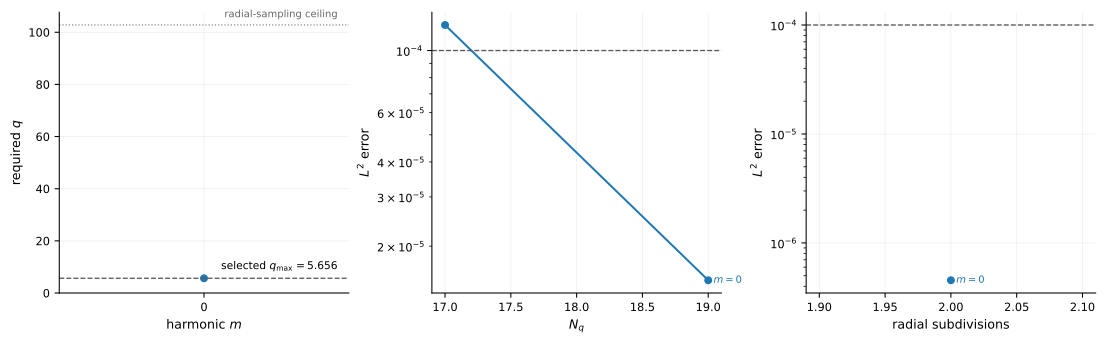
Harmonic-transform self-convergence diagnostics for the isotropic Gaussian example.#

Build the production transform without repeating the search:

field_c = hcal.transform(dec)

The calibrated object carries the same record, so the equivalent plot is also available later:

fig, axes = field_c.plot_convergence()

For a compact provenance record,

harmonic_record = hcal.to_dict()

contains the selected parameters, configured tolerances, and search history in JSON-serializable form.

A forward/inverse consistency diagnostic is also available:

print(f"round-trip relative L2: {field_c.roundtrip_error():.3e}")

roundtrip_error() checks consistency of the represented transform pair. It is not an independent error against the original continuum problem.

5. Calibrate the assembled interaction#

Interaction convergence depends on the transformed fields, kernel, and displacement set. Calibrate over the displacement domain that production will actually use.

calibration_delta = np.geomspace(1.0e-2, 1.0e2, 32)
calibration_deltas = np.column_stack(
    (calibration_delta, np.zeros_like(calibration_delta))
)

ical = Interaction.converge_parameters(
    calibration_deltas,
    field_c,
    field_c,
    coulomb,
    rtol=1.0e-4,
    atol=1.0e-12,
    method="gl4",
)

print("converged:", ical.converged)
print("selected parameters:", ical.parameters)

Interaction has the same inspection workflow as HarmonicTransform:

fig, axes = ical.plot_convergence()

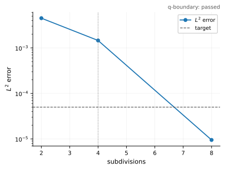
Interaction convergence diagnostics for the isotropic Gaussian example — Interaction self-convergence diagnostics for the isotropic Gaussian example.#

In all cases, the plot visualizes the internal search that produced the selected parameters.

Construct the interaction with the selected parameters without rerunning the search:

interaction_c = ical.interaction(
    calibration_deltas,
    field_c,
    field_c,
    coulomb,
)

The production object retains that record:

print(interaction_c.convergence is ical)
fig, axes = interaction_c.plot_convergence()
interaction_record = ical.to_dict()

True

The same pattern therefore applies at both numerical layers:

represent -> inspect -> calibrate -> plot convergence -> reuse -> save record

The complete tolerance semantics and failure diagnostics are developed in Convergence and diagnostics. The physical output arrays are explained in Evaluating interactions, and the full isotropic calculation is extended in Localized-state interactions in a 2D dielectric environment.

A full run of the executable script reports:

PETAL2D
retained modes: [0]
reconstruction error [%]: 1.176e-14
domain consistency: 0.99968873

HarmonicTransform
self-convergence satisfied: True
analytic relative L2 error: 7.486e-04
selected q_max: 5.655935
selected n_q: 19

Interaction
Coulomb self-convergence satisfied: True
Rytova-Keldysh self-convergence satisfied: True
delta=0.0  Coulomb=1.252579  RK=0.769954
delta=1.0  Coulomb=0.990611  RK=0.658185
delta=2.0  Coulomb=0.582827  RK=0.460529
delta=4.0  Coulomb=0.258812  RK=0.244462