Outputs and plotting#

QUARTIC2D keeps transformed harmonics, diagnostics, convergence records, and harmonic-pair interaction terms available after a calculation. Use the built-in helpers for numerical inspection before writing custom presentation plots.

HarmonicTransform inspection#

The primary transformed-field attributes are

print(field.m_values.tolist())
print(field.q.shape)
print(field.method)
print(field.interpolator)
print(field.diagnostics.healthy)

A specific harmonic is evaluated by calling the transformed field:

import numpy as np

q_eval = np.array([0.0, 1.0, 2.0])
F_m = field(0, q_eval)
print(F_m.shape)

(3,)

Plot transformed harmonics#

fig, axes = field.plot_harmonics()

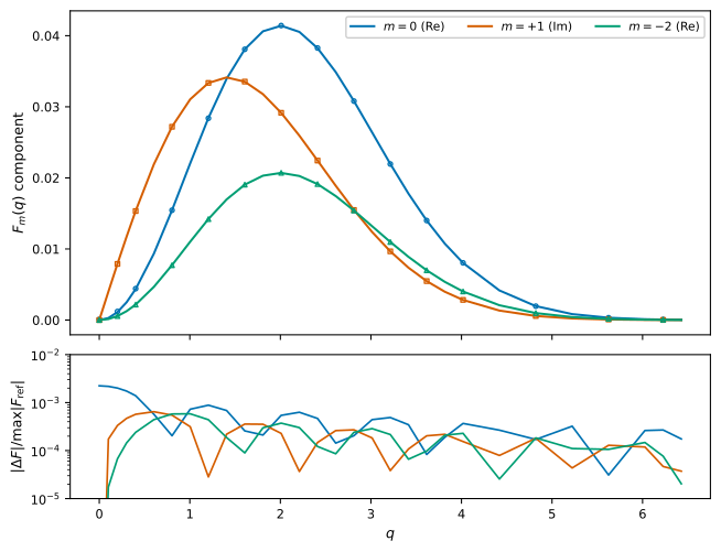
Harmonic transforms for a complex localized transition field — A representative transformed-harmonic figure produced by `field.plot_harmonics()`.#

This is the standard public helper for the real and imaginary parts of every retained \(F_m(q)\) profile. field.plot() provides the same profile figure as a compact convenience call.

Plot automatic convergence#

A field constructed from HarmonicTransform.converge_parameters(...) carries the corresponding search record:

fig, axes = field.plot_convergence()

The same plot is available before production construction from the result object itself:

fig, axes = calibration.plot_convergence()

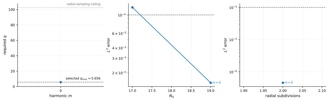
Harmonic-transform convergence diagnostics for the isotropic Gaussian example — A representative convergence figure returned by `plot_convergence()`.#

To request both profile and convergence figures from a calibrated field:

profiles, convergence = field.plot(show_convergence=True)

profiles and convergence are separate (fig, axes) pairs. Keeping the figures separate preserves readable panel sizes and lets each be saved or styled independently.

Inspect diagnostics and consistency numerically#

if not field.diagnostics.healthy:
    print(field.diagnostics.warning_message())

roundtrip = field.roundtrip_error()
print(f"round-trip relative L2: {roundtrip:.3e}")

roundtrip_error() is a forward/inverse consistency check on the represented transform, not an independent error against the original continuum problem.

Interaction outputs#

The main arrays are

print(interaction.V.shape)
print(interaction.V_mm.shape)
print(interaction.H_mm.shape)
print(interaction.Phi_mm.shape)

V is the assembled four-center matrix element over the displacement array. V_mm retains the angular-pair decomposition, H_mm contains the radial integrals, and Phi_mm contains the displacement-dependent angular factors.

If the interaction was created from InteractionConvergenceResult.interaction, the result is retained:

print(interaction.convergence)
fig, axes = interaction.plot_convergence()

The equivalent pre-production call is

fig, axes = interaction_calibration.plot_convergence()

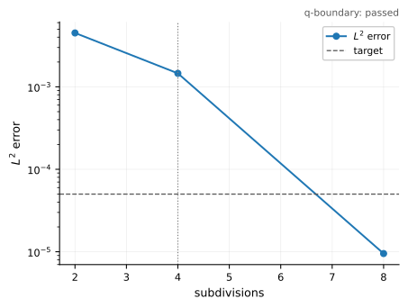
Interaction convergence diagnostics for the isotropic Gaussian example — A representative interaction convergence figure.#

The interaction convergence plot is method-aware: finite rules, FFTLog, and Ogata display the numerical checks relevant to their own parameter searches.

Plot a physical displacement sweep#

QUARTIC2D deliberately does not prescribe one plot for the physical observable, because a useful presentation depends on whether the problem is radial, anisotropic, real, or complex. A radial sweep can be plotted directly from V:

import matplotlib.pyplot as plt
import numpy as np

radius = np.linalg.norm(deltas, axis=1)
order = np.argsort(radius)

fig, ax = plt.subplots()
ax.plot(radius[order], interaction.V.real[order], "o-")
ax.set_xlabel(r"separation $\delta$")
ax.set_ylabel(r"$\mathrm{Re}\,U_{1234}$")
fig.tight_layout()

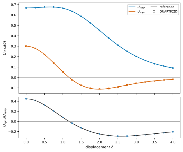
Direct and exchange matrix elements versus separation for normalized localized s and p_x orbitals — A physical displacement sweep built directly from the returned `V` arrays.#

For a complex matrix element, inspect real and imaginary parts or magnitude and phase according to the physical symmetry and gauge conventions of the orbital problem.

The direct/exchange example shows one radial presentation:

Harmonic-pair decomposition#

For one displacement, inspect every angular-pair contribution directly:

for i, m in enumerate(interaction.m_values1):
    for j, mp in enumerate(interaction.m_values2):
        value = interaction.V_mm[i, j, 0]
        print(f"m={m:2d}, mp={mp:2d}, V_mm={value}")

The numerical values depend on the field pair, kernel, and displacement. At zero displacement, only the angular combinations allowed by the Bessel factor survive. Finite displacement exposes the off-diagonal angular-pair structure.

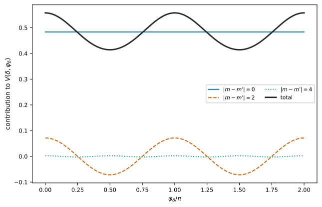
Harmonic-pair contributions to the anisotropic interaction — Grouping `V_mm` by \(|m-m'|\) is one useful way to expose how individual harmonic-pair channels build the total interaction.#

Preserve numerical provenance#

A quantitative result should retain enough information to reconstruct both the physical input and the numerical search:

orbital or transition-field definition and normalization.
PETAL2D settings, retained harmonics, and reconstruction diagnostics.
HarmonicTransform calibration or explicit transform parameters.
kernel definition, parameters, and units.
displacement vectors.
Interaction calibration or explicit production parameters.
requested self-convergence tolerances.
QUARTIC2D and PETAL2D versions.

The public convergence results make this straightforward:

harmonic_record = harmonic_calibration.to_dict()
interaction_record = interaction_calibration.to_dict()

These compact dictionaries are intended for logs, metadata files, and reproducibility records. Use InteractionConvergenceResult.to_dict(include_values=True) only when the full arrays from each refinement step are required.