Building Hamiltonians#

A second-quantized lattice Hamiltonian is a sum of one-body processes and interactions. For number-conserving models a useful general form is

\[ H=\sum_{ij}t_{ij}a_i^\dagger a_j +\frac{1}{2}\sum_{ij}V_{ij}n_in_j +H_{\mathrm{local}}+H_{\mathrm{exchange}}+\cdots, \]

where \(a_i\) is a fermionic or bosonic annihilation operator and \(t_{ij}\) may be complex. The Fock basis turns this operator into a finite matrix whose nonzero entries record which many-body configurations are connected by the Hamiltonian.

Hopping and density interactions#

For a spinless chain with nearest-neighbor hopping and repulsion,

\[ H=-t\sum_{\langle ij\rangle} (c_i^\dagger c_j+c_j^\dagger c_i) +V\sum_{\langle ij\rangle}n_in_j, \]

one can assemble the model term by term:

from edinpy import fermion as ed

L = 4
site = ed.DoF(L, name="site")
modes = ed.FermionModes(site)
sector = ed.NParticleSector(modes, N=2).build()

c = ed.set_notation(ed.Annihilation, modes)
cd = ed.set_notation(ed.Creation, modes)
n = ed.set_notation(ed.Number, modes)

t = 1.0
V = 0.5
H = 0

for i in range(L - 1):
    H += -t * (cd(i) * c(i + 1) + cd(i + 1) * c(i))
    H += V * n(i) * n(i + 1)

The same physical terms can be written with the standard helpers:

H = 0
for i in range(L - 1):
    H += ed.Hopping(i, i + 1, -t, modes)
    H += ed.DensityDensity(i, i + 1, V, modes)

Both forms produce the same operator expression. Handwritten products are useful for model-specific terms, while the helpers keep common conventions compact.

Hubbard interactions#

The spinful fermion Hubbard model is

\[ H=-t\sum_{\langle ij\rangle,\sigma} (c_{i\sigma}^\dagger c_{j\sigma}+\mathrm{h.c.}) +U\sum_i n_{i\uparrow}n_{i\downarrow}. \]

The local interaction penalizes a doublon, so increasing \(U/t\) suppresses charge fluctuations and leaves spin exchange as the low-energy process near half filling.

For the Bose-Hubbard model,

\[ H=-J\sum_{\langle ij\rangle} (b_i^\dagger b_j+\mathrm{h.c.}) +\frac{U}{2}\sum_i n_i(n_i-1), \]

where the factor \(n_i(n_i-1)/2\) counts on-site boson pairs. The corresponding terms are produced by fermion.Hubbard and boson.Hubbard. Longer-range density interactions, exchange, pair transfer, and custom operator products can be added to the same sum.

Spin exchange#

For two-component fermions or Schwinger bosons,

\[ S^+=a_\uparrow^\dagger a_\downarrow, \qquad S^-=a_\downarrow^\dagger a_\uparrow, \qquad S^z=\frac{1}{2}(n_\uparrow-n_\downarrow). \]

The Heisenberg interaction is

\[ J\mathbf S_i\cdot\mathbf S_j =J\left[ S_i^zS_j^z +\frac{1}{2}(S_i^+S_j^-+S_i^-S_j^+) \right]. \]

SpinPlus, SpinMinus, SpinX, SpinY, SpinZ, and HeisenbergExchange construct these terms directly. In a Schwinger-boson representation, the local boson-number constraint fixes the spin representation.

Conserved quantities and sector choice#

Every constraint used to define the basis must be respected by every Hamiltonian term. If a number operator \(Q\) is fixed in the sector, then

\[ [H,Q]=0 \]

is required for the Hamiltonian to remain inside that sector. The ordinary Hubbard model conserves both \(N_\uparrow\) and \(N_\downarrow\), so a sector with fixed spin populations is valid. A source term such as

\[ \Delta\left(c_{i\uparrow}^\dagger c_{i\downarrow}^\dagger + c_{i\downarrow}c_{i\uparrow}\right) \]

changes total particle number and cannot be represented completely inside one fixed-\(N\) block. The same check applies to layer, species, orbital, or other particle-number constraints.

For a new Hamiltonian, the smallest nontrivial system is often the most useful first calculation. At that size the complete matrix can be inspected, Hermiticity can be checked directly, and noninteracting or atomic limits can usually be compared with an independent result before moving to larger sectors.

Complex hopping amplitudes#

Peierls phases, twisted boundary conditions, and synthetic gauge fields introduce complex matrix elements. A single bond with phase \(\phi\) can be written

import numpy as np

phase = np.exp(1j * phi)
forward = phase * cd(0) * c(1)
H_phi = -t * (forward + forward.dag)

The Hermitian conjugate carries the complex-conjugate phase automatically through .dag.

Sparse matrix structure#

Once the operator and sector are specified,

hamiltonian = ed.Hamiltonian(H, sector)
matrix = hamiltonian.matrix

print(matrix.shape)
print(matrix.nnz)

returns the sparse CSC representation. In the Fock basis, diagonal density terms contribute to the diagonal, while hopping and exchange connect distinct configurations.

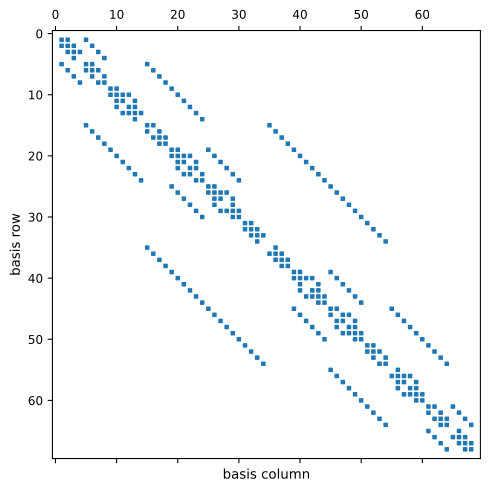
Sparse matrix pattern of the four-site half-filled Hubbard Hamiltonian — Sparse matrix pattern of the four-site open Hubbard model at half filling and \(U/t=4\). Hopping produces the off-diagonal connectivity, while the onsite interaction contributes diagonal matrix elements.#

For this four-site spinful problem the fixed-\(N\) sector has \(D=70\), so a dense representation contains \(D^2=4900\) entries. Only 294 entries are nonzero. The sparsity reflects locality in Fock space and is what makes Krylov methods useful beyond the range where dense diagonalization is reasonable.

For calculations that need only Hamiltonian-vector products, the matrix can also remain implicit through aslinearoperator() or eigsolve(matrix_free=True). The numerical choices are discussed in Numerical considerations.