Fock space, modes, and symmetry sectors

A many-body basis is specified by a set of one-particle modes and an occupation rule. For fermions each mode is either empty or occupied, while bosonic occupations are nonnegative integers. Exact diagonalization becomes practical only after all conserved quantum numbers that are relevant to the calculation have been used to reduce the Hilbert space.

Mode labels and ordering

A mode may carry several discrete labels, such as site, spin, orbital, layer, valley, or momentum. DoF stores one such label set. For a three-site spinful problem,

from edinpy import fermion as edf

site = edf.DoF(3, name="site")
spin = edf.DoF(2, name="spin", labels=("up", "down"))
modes = edf.FermionModes(site, spin)

print(modes.n_modes)
for p in range(modes.n_modes):
    print(p, modes.unravel(p))

6
0 (0, 0)
1 (1, 0)
2 (2, 0)
3 (0, 1)
4 (1, 1)
5 (2, 1)

With degree-of-freedom sizes \((d_0,d_1,\ldots)\), the flattened mixed-radix index is

\[ p=i_0+d_0i_1+d_0d_1i_2+\cdots. \]

Thus the first supplied degree of freedom varies fastest. resolve() maps physical labels to the flattened mode index, while unravel() performs the inverse map:

print(modes.resolve((2, 1)))
print(modes.unravel(4))

5
(1, 1)

For fermions, the ordering is also the ordering used in the Jordan-Wigner sign count for Fock-state operations. Once a mode convention has been chosen, the same modes object should be used for the basis, operators, Hamiltonian, and observables.

Fixed-particle-number sectors

If the Hamiltonian commutes with the total particle-number operator,

\[ [H,\hat N]=0, \]

the Hilbert space decomposes into independent sectors of fixed particle number \(N\). For \(M\) fermionic modes,

\[ D_F(M,N)=\binom{M}{N}, \]

while for \(M\) bosonic modes,

\[ D_B(M,N)=\binom{M+N-1}{N}. \]

The difference is purely combinatorial: fermions select \(N\) occupied modes, whereas bosons distribute \(N\) indistinguishable particles among \(M\) modes.

sector = edf.NParticleSector(modes, N=3).build()
print(sector.dimension)

20

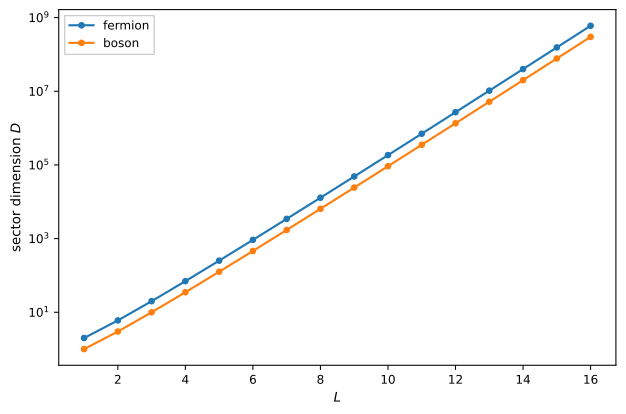
Fixed-particle-number dimensions for a half-filled spinful fermion chain and a unit-filled boson chain. The rapid combinatorial growth sets the basic system-size limit of exact diagonalization.

For the curves above, the fermionic problem has \(M=2L\) and \(N=L\), so \(D_F=\binom{2L}{L}\). The bosonic problem has \(M=L\) and \(N=L\), so \(D_B=\binom{2L-1}{L}\). Restricting to a conserved sector removes states that cannot mix under \(H\), but the remaining dimension still grows exponentially with lattice size.

Symmetry-constrained sectors

Additional conserved number operators produce smaller blocks. For a spin-conserving Hamiltonian,

\[ [H,\hat N_\uparrow]=[H,\hat N_\downarrow]=0, \qquad N=N_\uparrow+N_\downarrow. \]

The sector with fixed \((N_\uparrow,N_\downarrow)\) therefore has

\[ D=\binom{L}{N_\uparrow}\binom{L}{N_\downarrow} \]

for a spinful fermion lattice with \(L\) sites. With three sites, \(N_\uparrow=2\), and \(N_\downarrow=1\), the dimension is nine:

sector = (
    edf.NParticleSector(modes, N=3)
    .project_particles("spin", up=2, down=1)
    .build()
)
print(sector.dimension)

9

The same construction applies when particle number is separately conserved in a layer, orbital, species, or another labeled subspace. Multiple commuting constraints can be combined before the basis is built:

site = edf.DoF(4, name="site")
spin = edf.DoF(2, name="spin", labels=("up", "down"))
layer = edf.DoF(2, name="layer", labels=("top", "bottom"))
modes = edf.FermionModes(site, spin, layer)

sector = (
    edf.NParticleSector(modes, N=4)
    .project_particles("spin", up=2, down=2)
    .project_particles("layer", top=2, bottom=2)
    .build()
)

A constraint belongs in the basis only when the corresponding operator commutes with the Hamiltonian. Otherwise the projected space omits states that are dynamically coupled by the model.

Fock states and basis coefficients

A fermionic basis state is written

\[ |n_0n_1\ldots n_{M-1}\rangle, \qquad n_p\in\{0,1\}, \]

whereas a bosonic basis state allows \(n_p=0,1,2,\ldots\). The corresponding state constructors preserve these occupation rules:

fermion_state = edf.FockState(0b0101, n_modes=4)
print(fermion_state)

1 |0101>

from edinpy import boson as edb

boson_state = edb.FockState((2, 0, 1, 0))
print(boson_state)

1 |2,0,1,0>

An eigenstate in a finite sector is a superposition

\[ |\psi\rangle=\sum_\alpha A_\alpha|\alpha\rangle, \qquad P_\alpha=|A_\alpha|^2, \]

where \(|\alpha\rangle\) are Fock-basis states. The probability distribution \(P_\alpha\) often gives an immediate physical picture of the state.

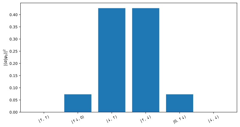
Ground-state Fock-basis probabilities of the half-filled Hubbard dimer at \(U/t=4\). The dominant configurations have one particle on each site, while hopping admixes doublon-hole configurations with smaller weight.

At positive \(U\), double occupation costs interaction energy. The ground state therefore concentrates on the two singly occupied configurations that form the spin singlet, while the finite doublon-hole weight records the charge fluctuations generated by hopping.

Numerical coefficient arrays can be attached to the sector basis with from_vector(), and eigenvectors returned by a Hamiltonian can be recovered as basis-aware states with eigenstate():

import numpy as np

coefficients = np.zeros(sector.dimension)
coefficients[0] = 1.0
psi = sector.from_vector(coefficients)

print(psi.norm())
print(psi.dag * psi)

1.0
1.0