Diagonalization and low-energy spectra

After choosing a finite symmetry sector, the stationary problem is

\[ H|\psi_n\rangle=E_n|\psi_n\rangle. \]

The useful part of the spectrum depends on the physics. Small clusters may require the complete eigensystem, for example to identify an exact multiplet. Larger many-body calculations usually target the ground state and a few low-lying excitations.

Complete spectra of small systems

The half-filled two-site Hubbard model provides a simple example. With two particles in four spin-orbitals, the sector dimension is six. Requesting k=None returns the complete spectrum:

energies, vectors = hamiltonian.eigsolve(k=None)
print(energies)
print(vectors.shape)

[-0.82842712  0.          0.          0.          4.          4.82842712]
(6, 6)

At \(U/t=4\), the three zero-energy states form the triplet. The remaining states belong to the singlet sector and include doublon-hole configurations.

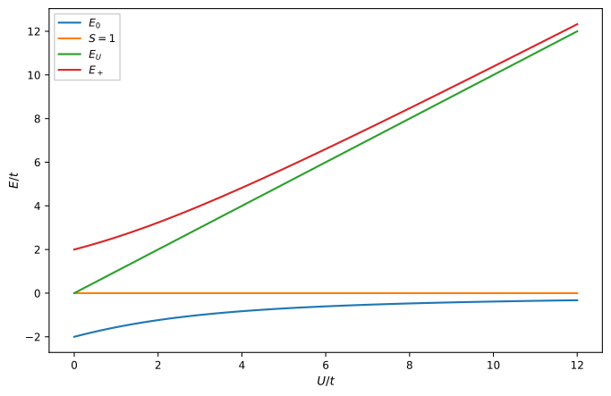
Complete half-filled Hubbard-dimer spectrum. The triplet remains at zero energy, while the singlet ground state approaches it from below as charge fluctuations are suppressed with increasing \(U/t\).

The singlet-triplet gap is

\[ \Delta_{ST}=E_T-E_0, \]

and in the strong-coupling limit,

\[ \Delta_{ST}\simeq\frac{4t^2}{U}. \]

This is the two-site form of antiferromagnetic superexchange.

Low-energy eigenpairs of larger sectors

When only a small part of the spectrum is needed, Krylov methods avoid the cost of computing every eigenvector. The six-site half-filled Hubbard ring, for example, already has a fixed-\(N\) dimension of 924. Its lowest excitation energies

\[ \Delta E_n=E_n-E_0 \]

can be obtained with

energies, vectors = hamiltonian.eigsolve(
    k=8,
    which="SA",
    tol=1e-10,
)

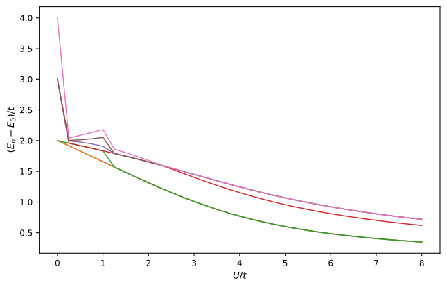
Lowest excitation energies of a six-site half-filled Hubbard ring. Several low-energy levels become closely spaced as the interaction grows, reflecting the emergence of a spin-dominated low-energy manifold.

which="SA" requests the smallest algebraic eigenvalues. LA, SM, and LM select the other standard ARPACK targets. The number of requested eigenpairs is k.

Krylov-space controls

For difficult spectra, the main iterative controls are

energies, vectors = hamiltonian.eigsolve(
    k=6,
    which="SA",
    tol=1e-12,
    maxiter=5000,
    ncv=32,
    v0=initial_vector,
)

tol controls the eigensolver convergence criterion. maxiter caps the number of Arnoldi/Lanczos iterations. ncv is the number of Lanczos vectors retained by ARPACK; increasing it can help when the targeted levels are clustered, at the cost of additional vector storage and orthogonalization. v0 supplies the starting vector and is useful in parameter sweeps when a nearby solution is already available.

Exact degeneracies require particular care. A converged iterative solve can return a valid subset of a degenerate eigenspace without spanning the entire multiplet. For small systems where the complete degenerate subspace is needed, dense diagonalization with k=None is the simplest choice.

Basis-aware eigenstates

The columns returned by eigsolve() are NumPy arrays. The corresponding Fock-space kets are available through

psi0 = hamiltonian.eigenstate(0)
psi1 = hamiltonian.eigenstate(1)

print(psi0.norm())
print(psi0.dag * psi1)

with typical output

0.9999999999999999
0.0

The basis-aware states can then be inserted directly into expectation values and correlation functions.

Residuals

For a numerical eigenpair \((E_n,v_n)\), the residual

\[ r_n=\|Hv_n-E_nv_n\|_2 \]

checks the eigensolver result:

import numpy as np

residual = np.linalg.norm(
    hamiltonian.matrix @ vectors[:, 0]
    - energies[0] * vectors[:, 0]
)

A small residual establishes convergence for the represented finite matrix. Physical convergence must still be examined with respect to system size, boundary conditions, local-state truncations, and any effective-model parameters.