Second-quantized operator algebra#
Many lattice Hamiltonians and observables are most compactly expressed in second quantization. The primitive creation and annihilation operators encode the particle statistics, while products and sums build the physical terms of the model.
Fermionic and bosonic algebra#
Fermionic operators satisfy
and bosonic operators satisfy
The number operator is
with \(a_p=c_p\) for fermions and \(a_p=b_p\) for bosons.
set_notation() is useful when many operators share the same mode space:
from edinpy import fermion as ed

modes = ed.FermionModes(ed.DoF(4, name="mode"))
c = ed.set_notation(ed.Annihilation, modes)
cd = ed.set_notation(ed.Creation, modes)
n = ed.set_notation(ed.Number, modes)

print(c(2))
print(cd(2))
print(n(2))
c[2]
c†[2]
n[2]
Action on Fock states#
For a fermionic state, annihilating mode \(p\) produces the sign
provided mode \(p\) is occupied. For example,
ket = ed.FockState(0b1010, n_modes=4)

print(c(1) * ket)
print(c(3) * ket)
print(cd(0) * c(3) * ket)
1 |1000>
-1 |0010>
-1 |0011>
For bosons,
from edinpy import boson as edb

modes_b = edb.BosonModes(edb.DoF(3, name="mode"))
b = edb.set_notation(edb.Annihilation, modes_b)
bd = edb.set_notation(edb.Creation, modes_b)
ket_b = edb.FockState((2, 0, 1))

print(b(0) * ket_b)
print(bd(1) * ket_b)
1.4142135623730951 |1,0,1>
1.0 |2,1,1>
These direct state operations are useful checks for fermionic signs, bosonic occupation factors, and short matrix elements derived by hand.
Sums, products, and Hermitian conjugation#
Ordinary Python arithmetic follows the written operator order:
hop = cd(0) * c(3)
interaction = 2.5 * n(0) * n(3)
H = -(hop + hop.dag) + interaction

print(H)
-1 c†[0] c[3] + -1 c†[3] c[0] + 2.5 n[0] n[3]
Thus cd(0) * c(3) is \(c_0^\dagger c_3\), and .dag reverses the product order and complex-conjugates scalar coefficients.
For a flux-threaded ring, differentiating the Hamiltonian with respect to the flux gives the persistent-current operator. For
with periodic boundary conditions, the current operator is
The second-quantized expression is
import numpy as np

L = 4
N = 2
t = 1.0
sector = ed.NParticleSector(modes, N=N).build()

phi = 0.4
phase = np.exp(1j * phi / L)
H = 0
I = 0

for j in range(L):
    k = (j + 1) % L
    hop = cd(j) * c(k)
    H += -t * (phase * hop + phase.conjugate() * hop.dag)
    I += (t / L) * (
        1j * phase * hop
        - 1j * phase.conjugate() * hop.dag
    )
The ground-state expectation value is then
hamiltonian = ed.Hamiltonian(H, sector)
hamiltonian.eigsolve(k=None)
psi0 = hamiltonian.eigenstate(0)
current = np.real(psi0.dag * I * psi0)
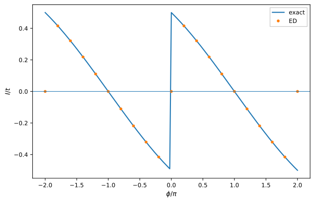
Persistent current of a half-filled four-site spinless fermion ring. Exact diagonalization reproduces the piecewise free-fermion result and its level-crossing discontinuities as the flux changes the occupied single-particle states.#
The sawtooth structure comes from crossings between many-body ground-state branches. The current is a custom response operator obtained from the Hamiltonian by differentiation with respect to flux.
Bras, kets, and matrix elements#
For basis-aware states, the textbook expressions
can be evaluated as
expectation = psi.dag * O * psi
transition = phi.dag * O * psi
overlap = phi.dag * psi
The method form psi.inner(phi) evaluates the same inner product as psi.dag * phi. Number-changing operators can also act on basis-aware states; the resulting symbolic state lies in the corresponding particle-number sector.
Common operator helpers#
Frequently used terms have compact constructors. For example,
is constructed by Hopping, while DensityDensity, Onsite, PairHopping, the spin operators, and HeisenbergExchange provide common interaction terms. The local Hubbard interaction is
for spinful fermions and
for bosons.
The exact signatures are collected in the Core API, Fermion API, and Boson API.