Numerical considerations

The cost of exact diagonalization is controlled first by the dimension of the symmetry sector and then by the representation used for repeated Hamiltonian operations. Numerical convergence of the eigensolver and convergence of the finite-system physics are separate questions and should be checked separately.

Reduce the Hilbert space first

For fixed particle number,

\[ D_F(M,N)=\binom{M}{N}, \qquad D_B(M,N)=\binom{M+N-1}{N}. \]

Every eigenvector and every Krylov vector has length \(D\). Fixing independently conserved particle numbers, such as \(N_\uparrow\) and \(N_\downarrow\) or particle numbers in separate layers or species, reduces both Hamiltonian construction and eigensolver memory. A constraint is valid only when its number operator commutes with the Hamiltonian.

For a half-filled spin-conserving Hubbard chain with even \(L\),

\[ N_\uparrow=N_\downarrow=L/2, \]

so the relevant \(S_z=0\) block has dimension

\[ D=\binom{L}{L/2}^2, \]

rather than \(\binom{2L}{L}\) for the complete fixed-\(N\) sector. The distinction becomes increasingly important as \(L\) grows.

Sparse matrices and matrix-free operators

A sparse CSC matrix is useful when matrix elements must be inspected, when the same matrix is reused by several numerical routines, or when an external method expects an explicit sparse object:

matrix = hamiltonian.matrix

For a few extremal eigenpairs, the Hamiltonian can instead be applied as a linear operator:

energies, vectors = hamiltonian.eigsolve(
    k=4,
    which="SA",
    matrix_free=True,
    execution="numpy",
)

Matrix-free execution avoids storing the sparse Hamiltonian. The Krylov basis remains present, so the eigensolver still stores vectors of length \(D\).

A small problem can be used to verify that the two representations describe the same finite Hamiltonian:

import numpy as np

rng = np.random.default_rng(1234)
x = rng.normal(size=sector.dimension)

H_sparse = hamiltonian.matrix
H_linear = hamiltonian.aslinearoperator(execution="numpy")

np.testing.assert_allclose(
    H_sparse @ x,
    H_linear @ x,
    rtol=1e-12,
    atol=1e-12,
)

This comparison is useful when a new operator contains several hopping, exchange, or complex-valued terms because it checks the complete Hamiltonian action on a vector rather than one matrix element at a time.

Matrix-free execution modes

The execution argument selects the implementation used for repeated Hamiltonian-vector products:

value	typical use
numpy	small and moderate calculations; numerical baseline for compiled paths
numba-serial	repeated supported products large enough to amortize JIT compilation
numba-parallel	large supported workloads with sufficient work per basis state for threading
mixed	conservative automatic selection for the particle statistics

The first call to a Numba path includes JIT compilation and should not be included in steady-state timing. Parallel execution is workload dependent: thread overhead can dominate a moderate sector even when a larger sector scales well. Representative measurements are given in Performance validation.

Explicit Numba modes are strict. An unsupported basis or operator structure raises an error rather than silently changing the requested execution mode.

Krylov-space memory

For either sparse or matrix-free Hamiltonians, ARPACK stores a Krylov basis. In double precision, one real vector requires approximately

\[ 8D\ \mathrm{bytes}, \]

and one complex vector approximately

\[ 16D\ \mathrm{bytes}. \]

A lower estimate for storing ncv Krylov vectors is therefore

\[ M_{\mathrm{Krylov}}\sim bD\,n_{cv}, \]

with \(b=8\) or \(16\) bytes before solver work arrays and orthogonalization storage are included. Increasing ncv can improve convergence for clustered eigenvalues but increases this memory cost.

Numerical convergence of an eigenpair

For a Ritz pair \((E_n,v_n)\),

\[ r_n=\|Hv_n-E_nv_n\|_2 \]

measures convergence of the represented finite eigenproblem. Residuals should be checked at representative points in a parameter sweep, especially near level crossings or closely spaced multiplets. Repeating selected calculations with tighter tol, larger ncv, or a different initial vector provides a direct stability check.

Hermiticity and known limits probe different errors. For a newly constructed model, useful checks include

• \(H=H^\dagger\) for a Hermitian problem;

• the noninteracting limit when the many-body result can be reconstructed from one-particle levels;

• the atomic or decoupled limit when hopping is set to zero;

• agreement between literal operator products and a standard helper for the same term;

• agreement between sparse and matrix-free Hamiltonian action on a small sector.

Finite-size convergence

A small residual does not imply that the finite cluster represents the thermodynamic limit. System size, boundary conditions, and the chosen symmetry sector remain part of the physical calculation.

For the half-filled open Hubbard chain at \(U/t=4\), the ground-state energy density

\[ e_0(L)=\frac{E_0(L)}{Lt} \]

can be followed through even chains with \(N_\uparrow=N_\downarrow=L/2\). The thermodynamic value from the Lieb-Wu solution is

\[ e_0(\infty) =-4\int_0^\infty \frac{J_0(\omega)J_1(\omega)} {\omega\left[1+e^{2\omega}\right]} \,d\omega \simeq -0.573729. \]

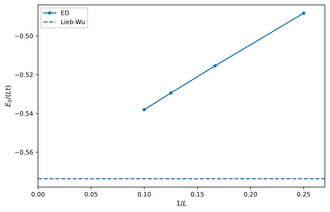
Ground-state energy density of half-filled open Hubbard chains at \(U/t=4\). The finite-system values approach the Lieb-Wu thermodynamic result as \(1/L\) decreases.

Convergence must be assessed separately for each observable. Correlation lengths, excitation gaps, order parameters, and boundary-sensitive observables can require different sizes. The complete calculation and sector construction are given in Half-filled Hubbard ring: Mott correlations on a finite cluster.

For finite-system studies, the following checks address distinct sources of error:

• increase \(L\) before assigning thermodynamic meaning to a crossover or gap;

• compare boundary conditions when shell effects or edge physics can matter;

• increase any explicit local bosonic occupation cutoff used outside a fixed-\(N\) construction;

• preserve every conserved quantity used to define a symmetry-constrained sector;

• resolve exact degeneracies with the relevant symmetry sector or a complete small-block diagonalization;

• compare selected parameter points against tighter eigensolver settings.

These checks determine whether the numerical eigenpair is accurate and whether the finite Hamiltonian supports the physical conclusion drawn from it.