Observables and correlation functions

Eigenvalues identify the energy scales of a finite system; expectation values and correlations identify the character of the corresponding states. Local observables probe charge and spin fluctuations, while correlation functions reveal how those fluctuations are organized in real and momentum space.

The fermionic examples below use a half-filled Hubbard system with UP = 0 and DOWN = 1.

Expectation values

For a normalized state \(|\psi\rangle\),

\[ \langle O\rangle=\langle\psi|O|\psi\rangle. \]

With a basis-aware eigenstate,

psi0 = hamiltonian.eigenstate(0)
value = psi0.dag * O * psi0

is evaluated in code as shown above.

For the Hubbard model, two elementary local quantities are the density

\[ n_i=n_{i\uparrow}+n_{i\downarrow} \]

and the double-occupancy operator

\[ D_i=n_{i\uparrow}n_{i\downarrow}. \]

n = ed.set_notation(ed.Number, modes)

n_i = n(i, UP) + n(i, DOWN)
D_i = n(i, UP) * n(i, DOWN)

mean_density = psi0.dag * n_i * psi0
mean_double = psi0.dag * D_i * psi0

For the two-site model it is useful to monitor the total double occupancy

\[ D=\sum_i\langle n_{i\uparrow}n_{i\downarrow}\rangle. \]

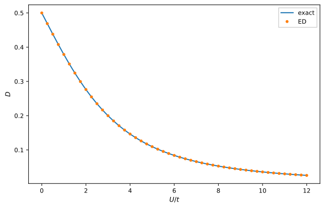
Total double occupancy of the half-filled Hubbard dimer. Repulsive interactions continuously suppress doublon-hole admixture as the ground state evolves toward the singly occupied spin sector.

At \(U=0\), hopping produces substantial charge fluctuations. Increasing \(U/t\) penalizes doublons, and the corresponding weight moves into singly occupied configurations.

Real-space spin correlations

At half filling, define the local spin projection

\[ S_i^z=\frac{1}{2}(n_{i\uparrow}-n_{i\downarrow}). \]

The translationally averaged equal-time spin correlation is

\[ C_s(r)=\frac{1}{L}\sum_i \langle S_i^zS_{i+r}^z\rangle. \]

The local operators can be built once,

Sz = [
    ed.SpinZ((i, UP), (i, DOWN), modes)
    for i in range(L)
]

and the correlation function can be evaluated for any separation:

def translational_correlation(psi, local_operators, r):
    L = len(local_operators)
    return sum(
        psi.dag
        * local_operators[i]
        * local_operators[(i + r) % L]
        * psi
        for i in range(L)
    ) / L

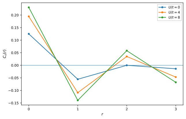
Spin correlations \(C_s(r)\) of a six-site half-filled Hubbard ring. Repulsion strengthens the alternating sign pattern expected from antiferromagnetic superexchange.

The finite ring contains only a few separations, so the curve is not an order-parameter extrapolation. Its value is local: increasing \(U/t\) suppresses charge motion and enhances antiferromagnetic correlations between the remaining spins.

Connected charge correlations

At half filling,

\[ \delta n_i=n_i-1, \]

and the connected charge correlation is

\[ C_c(r)=\frac{1}{L}\sum_i \langle\delta n_i\,\delta n_{i+r}\rangle. \]

The operator list is

delta_n = [
    n(i, UP) + n(i, DOWN) - 1
    for i in range(L)
]

and the same translational_correlation() function evaluates \(C_c(r)\).

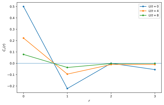
Connected charge correlations \(C_c(r)\) of a six-site half-filled Hubbard ring. The correlation amplitude decreases rapidly with increasing \(U/t\) as double occupancy and charge transfer are suppressed.

The opposite evolution of the spin and charge curves is a characteristic finite-system signature of the repulsive half-filled Hubbard model: spin fluctuations survive in the low-energy sector while charge fluctuations become increasingly costly.

Structure factors

For local operators \(O_j\), define

\[ O_q=\sum_{j=0}^{L-1}e^{-iqj}O_j \]

and the equal-time structure factor

\[ S_O(q)=\frac{1}{L}\langle O_q^\dagger O_q\rangle. \]

A single routine evaluates this definition for any list of local operators:

import numpy as np


def structure_factor(psi, local_operators, q):
    L = len(local_operators)
    O_q = sum(
        (
            np.exp(-1j * q * j) * operator
            for j, operator in enumerate(local_operators)
        ),
        start=0,
    )
    return np.real(psi.dag * O_q.dag * O_q * psi) / L

For \(O_j=S_j^z\), this gives the spin structure factor \(S_s(q)\).

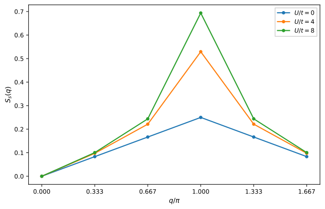
Spin structure factor of a six-site half-filled Hubbard ring. Spectral weight accumulates at the staggered wavevector \(q=\pi\) as repulsion strengthens antiferromagnetic correlations.

For \(O_j=\delta n_j\), the same function gives the connected charge structure factor \(S_c(q)\).

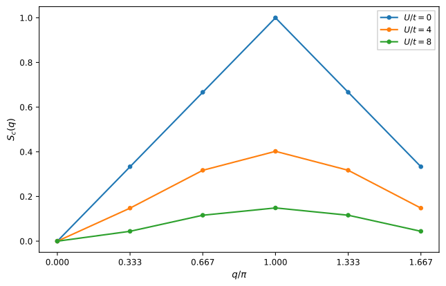
Connected charge structure factor of a six-site half-filled Hubbard ring. Repulsion suppresses charge fluctuations throughout the Brillouin zone, including the staggered component at \(q=\pi\).

A model-specific order parameter is implemented by changing the operator list rather than changing the correlation routine. For example, the onsite pair field

\[ \Delta_j=c_{j\downarrow}c_{j\uparrow} \]

can be constructed as

pair = [c(i, DOWN) * c(i, UP) for i in range(L)]
P_q = structure_factor(psi0, pair, q)

The operator list may instead contain bond, orbital, excitonic, or other composite operators; the structure-factor routine then measures the corresponding channel.

One-body density matrix and natural occupations

For either particle statistics, the one-body density matrix is

\[ \rho^{(1)}_{ij}=\langle a_i^\dagger a_j\rangle. \]

A direct implementation is

def one_body_density_matrix(psi, creation, annihilation, n_modes):
    rho = np.empty((n_modes, n_modes), dtype=complex)
    for i in range(n_modes):
        for j in range(n_modes):
            rho[i, j] = (
                psi.dag * creation(i) * annihilation(j) * psi
            )
    return rho

For a bosonic state, the eigenvalues \(\lambda_\alpha\) of \(\rho^{(1)}\) are the natural occupations. In a finite system with \(N\) particles, the largest natural occupation defines

\[ f_c=\frac{\lambda_{\max}}{N}. \]

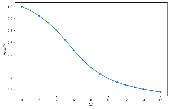
Largest natural occupation divided by \(N\) for a six-site unit-filled Bose-Hubbard ring. Increasing \(U/J\) depletes the dominant natural orbital as the finite system crosses from a delocalized regime toward interaction-localized number states.

This finite ring does not locate the thermodynamic superfluid-Mott transition. It does show how the one-body density matrix changes as coherence is lost, and the same calculation scales naturally to other finite bosonic lattices accessible to exact diagonalization.

The accompanying onsite number variance,

\[ \Delta n^2=\frac{1}{L}\sum_i \left(\langle n_i^2\rangle-\langle n_i\rangle^2\right), \]

provides the complementary local measure:

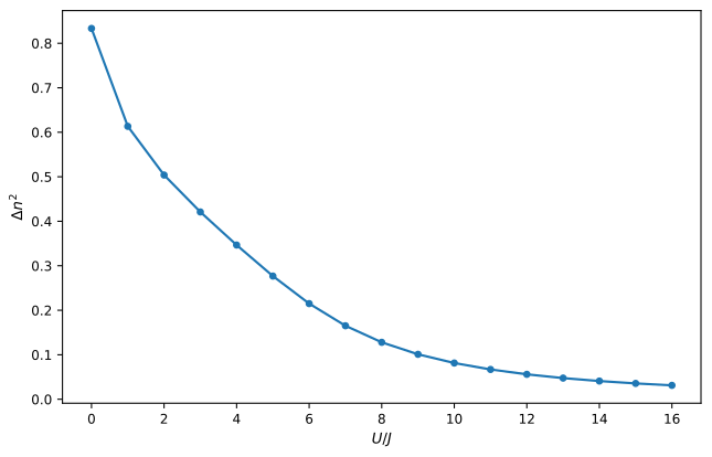
Mean onsite number variance of a six-site unit-filled Bose-Hubbard ring. Repulsion narrows the local occupation distribution and suppresses number fluctuations.

The simultaneous decrease of \(f_c\) and \(\Delta n^2\) gives two views of the same finite-size crossover: coherence is reduced in the one-body density matrix while site occupations become more sharply defined.

Transition matrix elements

Spectroscopy and response calculations often require

\[ \langle\psi_m|O|\psi_n\rangle. \]

Once the relevant eigenstates have been retained,

psi0 = hamiltonian.eigenstate(0)
psi1 = hamiltonian.eigenstate(1)
matrix_element = psi1.dag * O * psi0

computes the transition amplitude directly. Within an exactly degenerate eigenspace, individual eigenvectors depend on the basis returned by the diagonalizer, so transition amplitudes should be organized by the conserved quantum numbers relevant to the physical response.